Financial Modeling the Crisis Terry Marsh Quantal International

Financial Modeling & the Crisis Terry Marsh Quantal International Inc. 19 th Annual Conference of the PBFEAM Friday, July 8 , 2011 Taipei

Joint Work, Background Papers n n Work is with Paul Pfleiderer http: //www. quantal. com/Research

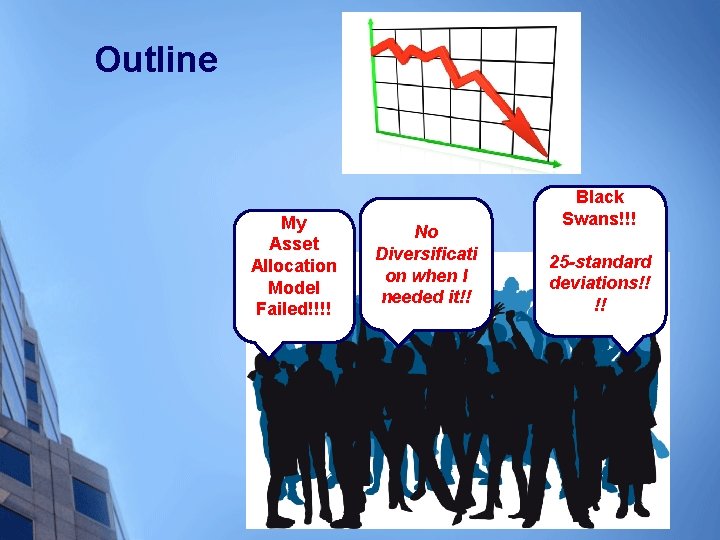
Outline My Asset Allocation Model Failed!!!! No Diversificati on when I needed it!! Black Swans!!! 25 -standard deviations!! !!

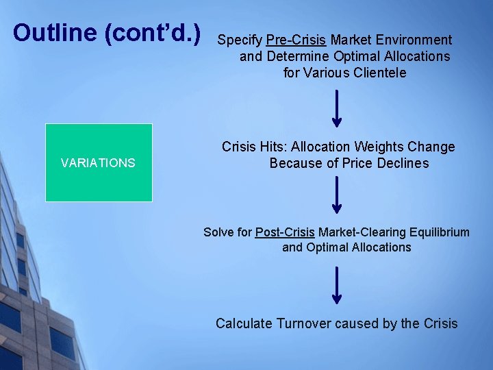
Outline (cont’d. ) BASE VARIATIONS CASE Specify Pre-Crisis Market Environment and Determine Optimal Allocations for Various Clientele Crisis Hits: Allocation Weights Change Because of Price Declines Solve for Post-Crisis Market-Clearing Equilibrium and Optimal Allocations Calculate Turnover caused by the Crisis

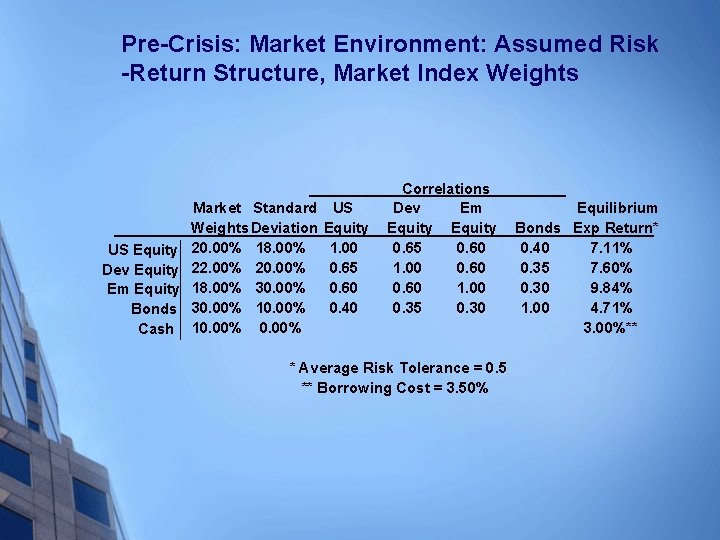
Pre-Crisis: Market Environment: Assumed Risk -Return Structure, Market Index Weights US Equity Dev Equity Em Equity Bonds Cash Market Standard Weights Deviation 20. 00% 18. 00% 22. 00% 20. 00% 18. 00% 30. 00% 10. 00% US Equity 1. 00 0. 65 0. 60 0. 40 Correlations Dev Em Equity 0. 65 0. 60 1. 00 0. 35 0. 30 * Average Risk Tolerance = 0. 5 ** Borrowing Cost = 3. 50% Equilibrium Bonds Exp Return* 0. 40 7. 11% 0. 35 7. 60% 0. 30 9. 84% 1. 00 4. 71% 3. 00%**

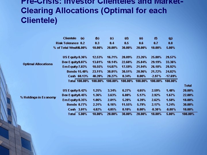
Pre-Crisis: Investor Clienteles and Market. Clearing Allocations (Optimal for each Clientele) Clientele (a) Risk Tolerance 0. 2 % of Total Wealth 5. 00% Optimal Allocations % Holdings in Economy US Equity 8. 36% Dev Equity 9. 07% Em Equity 7. 03% Bonds 15. 40% Cash 60. 13% Total 100. 00% US Equity 0. 42% Dev Equity 0. 45% Em Equity 0. 35% Bonds 0. 77% Cash 3. 01% Total 5. 00% (b) 0. 3 10. 00% (c) 0. 4 20. 00% (d) 0. 5 30. 00% (e) 0. 6 20. 00% (f) 0. 7 10. 00% (g) 0. 8 5. 00% 12. 53% 13. 61% 10. 55% 23. 11% 40. 20% 100. 00% 16. 71% 18. 14% 14. 07% 30. 81% 20. 27% 100. 00% 20. 89% 22. 68% 17. 59% 38. 51% 0. 34% 100. 00% 23. 26% 25. 84% 21. 94% 28. 96% 0. 00% 100. 00% 25. 88% 29. 19% 26. 18% 21. 72% -2. 97% 100. 00% 29. 57% 33. 36% 29. 92% 24. 82% -17. 69% 100. 00% 1. 25% 1. 36% 1. 06% 2. 31% 4. 02% 10. 00% 3. 34% 3. 63% 2. 81% 6. 16% 4. 05% 20. 00% 6. 27% 6. 80% 5. 28% 11. 55% 0. 10% 30. 00% 4. 65% 5. 17% 4. 39% 5. 79% 0. 00% 2. 59% 2. 92% 2. 62% 2. 17% -0. 30% 10. 00% 1. 48% 1. 67% 1. 50% 1. 24% -0. 88% 5. 00% Total 20. 00% 22. 00% 18. 00% 30. 00% 100. 00%

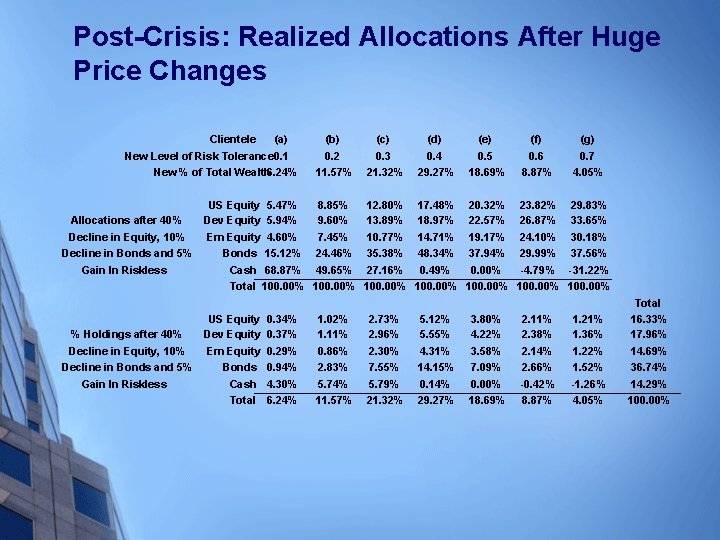
Post-Crisis: Realized Allocations After Huge Price Changes Clientele (a) New Level of Risk Tolerance 0. 1 New % of Total Wealth 6. 24% Allocations after 40% Decline in Equity, 10% Decline in Bonds and 5% Gain In Riskless % Holdings after 40% Decline in Equity, 10% Decline in Bonds and 5% Gain In Riskless (c) 0. 3 21. 32% (d) 0. 4 29. 27% (e) 0. 5 18. 69% (f) 0. 6 8. 87% (g) 0. 7 4. 05% US Equity 5. 47% 8. 85% 12. 80% Dev Equity 5. 94% 9. 60% 13. 89% Em Equity 4. 60% 7. 45% 10. 77% Bonds 15. 12% 24. 46% 35. 38% Cash 68. 87% 49. 65% 27. 16% Total 100. 00% 17. 48% 18. 97% 14. 71% 48. 34% 0. 49% 100. 00% 20. 32% 22. 57% 19. 17% 37. 94% 0. 00% 100. 00% 23. 82% 26. 87% 24. 10% 29. 99% -4. 79% 100. 00% 29. 83% 33. 65% 30. 18% 37. 56% -31. 22% 100. 00% US Equity Dev Equity Em Equity Bonds Cash Total 0. 34% 0. 37% 0. 29% 0. 94% 4. 30% 6. 24% (b) 0. 2 11. 57% 1. 02% 1. 11% 0. 86% 2. 83% 5. 74% 11. 57% 2. 73% 2. 96% 2. 30% 7. 55% 5. 79% 21. 32% 5. 12% 5. 55% 4. 31% 14. 15% 0. 14% 29. 27% 3. 80% 4. 22% 3. 58% 7. 09% 0. 00% 18. 69% 2. 11% 2. 38% 2. 14% 2. 66% -0. 42% 8. 87% 1. 21% 1. 36% 1. 22% 1. 52% -1. 26% 4. 05% Total 16. 33% 17. 96% 14. 69% 36. 74% 14. 29% 100. 00%

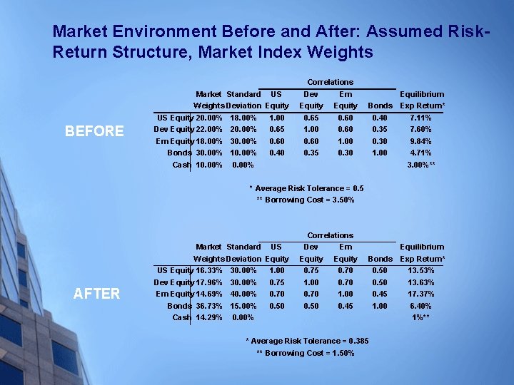
Market Environment Before and After: Assumed Risk. Return Structure, Market Index Weights BEFORE Market Standard US Weights Deviation Equity US Equity 20. 00% 18. 00% 1. 00 Dev Equity 22. 00% 20. 00% 0. 65 Em Equity 18. 00% 30. 00% 0. 60 Bonds 30. 00% 10. 00% 0. 40 Cash 10. 00% Correlations Dev Em Equity 0. 65 0. 60 1. 00 0. 35 0. 30 Equilibrium Bonds Exp Return* 0. 40 7. 11% 0. 35 7. 60% 0. 30 9. 84% 1. 00 4. 71% 3. 00%** * Average Risk Tolerance = 0. 5 ** Borrowing Cost = 3. 50% AFTER Market Standard US Weights Deviation Equity US Equity 16. 33% 30. 00% 1. 00 Dev Equity 17. 96% 30. 00% 0. 75 Em Equity 14. 69% 40. 00% 0. 70 Bonds 36. 73% 15. 00% 0. 50 Cash 14. 29% 0. 00% Correlations Dev Em Equity 0. 75 0. 70 1. 00 0. 50 0. 45 Equilibrium Bonds Exp Return* 0. 50 13. 53% 0. 50 13. 63% 0. 45 17. 37% 1. 00 6. 40% 1%** * Average Risk Tolerance = 0. 385 ** Borrowing Cost = 1. 50%

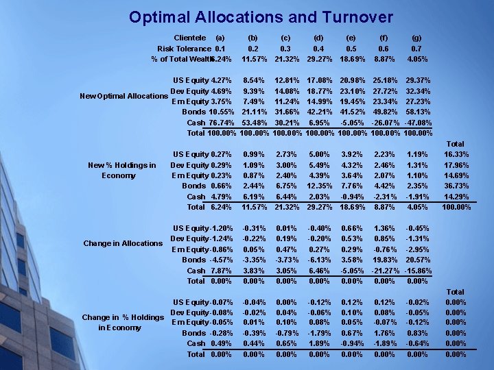
Optimal Allocations and Turnover Clientele (a) Risk Tolerance 0. 1 % of Total Wealth 6. 24% US Equity 4. 27% Dev Equity 4. 69% New Optimal Allocations Em Equity 3. 75% Bonds 10. 55% Cash 76. 74% Total 100. 00% New % Holdings in Economy Change in Allocations (b) (c) (d) (e) 0. 2 0. 3 0. 4 0. 5 11. 57% 21. 32% 29. 27% 18. 69% 8. 54% 9. 39% 7. 49% 21. 11% 53. 48% 100. 00% 12. 81% 14. 08% 11. 24% 31. 66% 30. 21% 100. 00% 17. 08% 18. 77% 14. 99% 42. 21% 6. 95% 100. 00% 20. 98% 23. 10% 19. 45% 41. 52% -5. 05% 100. 00% US Equity 0. 27% Dev Equity 0. 29% Em Equity 0. 23% Bonds 0. 66% Cash 4. 79% Total 6. 24% 0. 99% 2. 73% 5. 00% 3. 92% 1. 09% 3. 00% 5. 49% 4. 32% 0. 87% 2. 40% 4. 39% 3. 64% 2. 44% 6. 75% 12. 35% 7. 76% 6. 19% 6. 44% 2. 03% -0. 94% 11. 57% 21. 32% 29. 27% 18. 69% US Equity -1. 20% Dev Equity-1. 24% Em Equity-0. 86% Bonds -4. 57% Cash 7. 87% Total 0. 00% -0. 31% -0. 22% 0. 05% -3. 35% 3. 83% 0. 00% US Equity -0. 07% Dev Equity-0. 08% Change in % Holdings Em Equity-0. 05% in Economy Bonds -0. 28% Cash 0. 49% Total 0. 00% -0. 04% -0. 02% 0. 01% -0. 39% 0. 44% 0. 00% 0. 01% 0. 19% 0. 47% -3. 73% 3. 05% 0. 00% 0. 04% 0. 10% -0. 79% 0. 65% 0. 00% -0. 40% -0. 20% 0. 27% -6. 13% 6. 46% 0. 00% -0. 12% -0. 06% 0. 08% -1. 79% 1. 89% 0. 00% (f) 0. 6 8. 87% (g) 0. 7 4. 05% 25. 18% 27. 72% 23. 34% 49. 82% -26. 07% 100. 00% 29. 37% 32. 34% 27. 23% 58. 13% -47. 08% 100. 00% 2. 23% 2. 46% 2. 07% 4. 42% -2. 31% 8. 87% 1. 19% 1. 31% 1. 10% 2. 35% -1. 91% 4. 05% Total 16. 33% 17. 96% 14. 69% 36. 73% 14. 29% 100. 00% 0. 66% 1. 36% -0. 45% 0. 53% 0. 85% -1. 31% 0. 29% -0. 76% -2. 95% 3. 58% 19. 83% 20. 57% -5. 05% -21. 27% -15. 86% 0. 00% 0. 12% 0. 10% 0. 05% 0. 67% -0. 94% 0. 00% 0. 12% 0. 08% -0. 07% 1. 76% -1. 89% 0. 00% -0. 02% -0. 05% -0. 12% 0. 83% -0. 64% 0. 00% Total 0. 00%

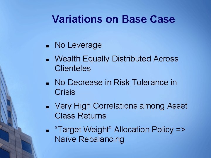
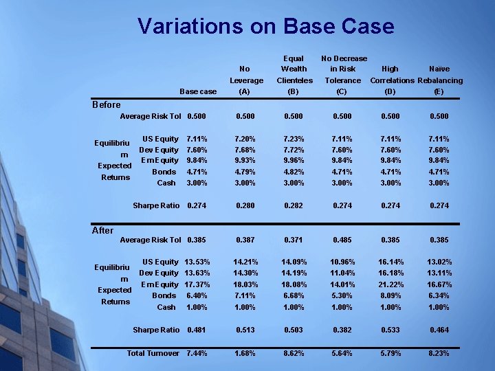
Variations on Base Case n n n No Leverage Wealth Equally Distributed Across Clienteles No Decrease in Risk Tolerance in Crisis Very High Correlations among Asset Class Returns “Target Weight” Allocation Policy => Naïve Rebalancing

Variations on Base Case Base case No Leverage (A) Equal Wealth Clienteles (B) No Decrease in Risk High Naïve Tolerance Correlations Rebalancing (C) (D) (E) 0. 500 Before Average Risk Tol 0. 500 US Equity Dev Equity Em Equity Bonds Cash 7. 11% 7. 60% 9. 84% 4. 71% 3. 00% 7. 20% 7. 68% 9. 93% 4. 79% 3. 00% 7. 23% 7. 72% 9. 96% 4. 82% 3. 00% 7. 11% 7. 60% 9. 84% 4. 71% 3. 00% Sharpe Ratio 0. 274 0. 280 0. 282 0. 274 Average Risk Tol 0. 385 0. 387 0. 371 0. 485 0. 385 14. 21% 14. 30% 18. 03% 7. 11% 1. 00% 14. 09% 14. 19% 18. 08% 6. 68% 1. 00% 10. 96% 11. 04% 14. 01% 5. 30% 1. 00% 16. 14% 16. 18% 21. 22% 8. 09% 1. 00% 13. 02% 13. 11% 16. 67% 6. 34% 1. 00% 0. 481 0. 513 0. 503 0. 382 0. 533 0. 464 Total Turnover 7. 44% 1. 68% 8. 62% 5. 64% 5. 79% 8. 23% Equilibriu m Expected Returns After Equilibriu m Expected Returns US Equity 13. 53% Dev Equity 13. 63% Em Equity 17. 37% Bonds 6. 40% Cash 1. 00% Sharpe Ratio

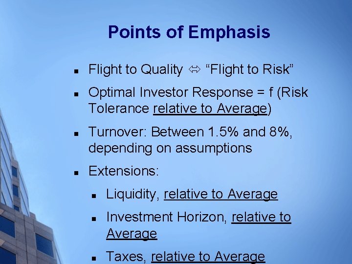
Points of Emphasis n n Flight to Quality “Flight to Risk” Optimal Investor Response = f (Risk Tolerance relative to Average) Turnover: Between 1. 5% and 8%, depending on assumptions Extensions: n n n Liquidity, relative to Average Investment Horizon, relative to Average Taxes, relative to Average

Related Points n n n Good Companies ≠ Good Investments Low Property Taxes ≠ Low House Prices Publicly Listed Private Equity Firms ≠ “Private Equity for Everyman” …. .

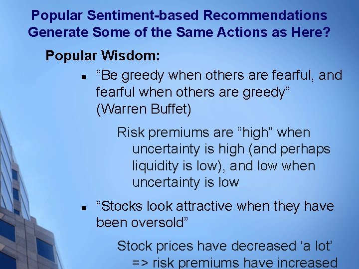
Popular Sentiment-based Recommendations Generate Some of the Same Actions as Here? Popular Wisdom: n “Be greedy when others are fearful, and fearful when others are greedy” (Warren Buffet) Risk premiums are “high” when uncertainty is high (and perhaps liquidity is low), and low when uncertainty is low n “Stocks look attractive when they have been oversold” Stock prices have decreased ‘a lot’ => risk premiums have increased

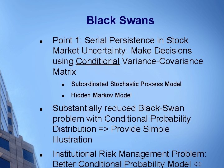
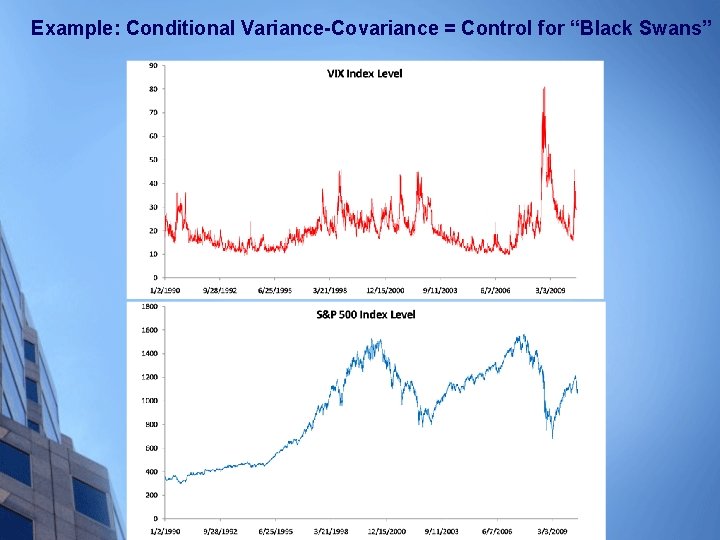
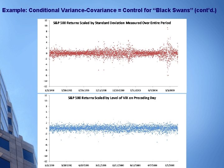
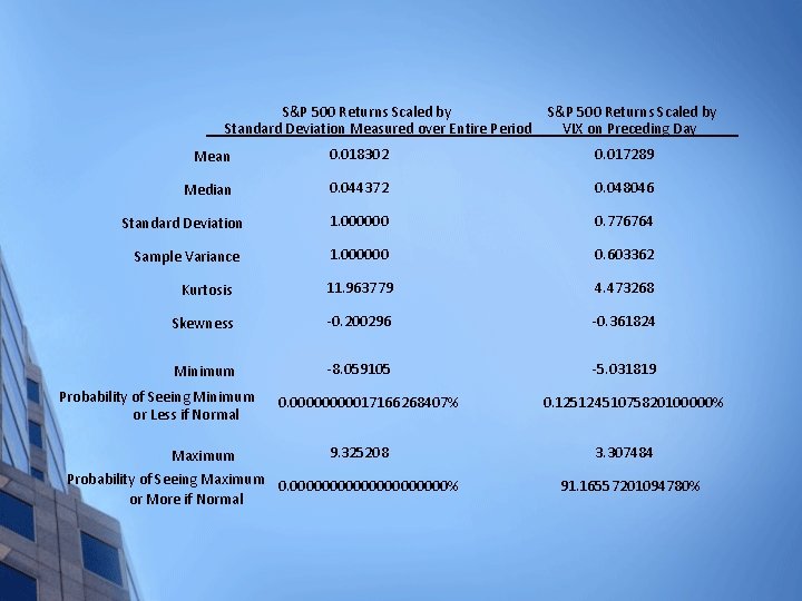
Black Swans n n n Point 1: Serial Persistence in Stock Market Uncertainty: Make Decisions using Conditional Variance-Covariance Matrix n Subordinated Stochastic Process Model n Hidden Markov Model Substantially reduced Black-Swan problem with Conditional Probability Distribution => Provide Simple Illustration Institutional Risk Management Problem: Better Conditional Probability Model

Example: Conditional Variance-Covariance = Control for “Black Swans”

Example: Conditional Variance-Covariance = Control for “Black Swans” (cont’d. )

S&P 500 Returns Scaled by Standard Deviation Measured over Entire Period S&P 500 Returns Scaled by VIX on Preceding Day Mean 0. 018302 0. 017289 Median 0. 044372 0. 048046 Standard Deviation 1. 000000 0. 776764 Sample Variance 1. 000000 0. 603362 Kurtosis 11. 963779 4. 473268 Skewness -0. 200296 -0. 361824 Minimum -8. 059105 -5. 031819 Probability of Seeing Minimum or Less if Normal Maximum 0. 0000017166268407% 9. 325208 Probability of Seeing Maximum 0. 0000000000% or More if Normal 0. 12512451075820100000% 3. 307484 91. 16557201094780%

Interesting Questions re “Black Swans”? n Who buys insurance against “black swan” events, who supplies this insurance, who self-insures, when does the insurance market “break down”…. etc.