Financial Management 5 Cost of capital WACC Model

Financial Management 5. Cost of capital. WACC Model. 6. Time Value of Money. 7. Basic Model of Capital Assets Valuation. Liliya N. Zhilina, World Economy and Inrernational Relations Department, Vladivostok State University of Economic and Services (VSUES). liliya. zhilina@vvsu. ru

5. Cost of Capital. WACC Model.

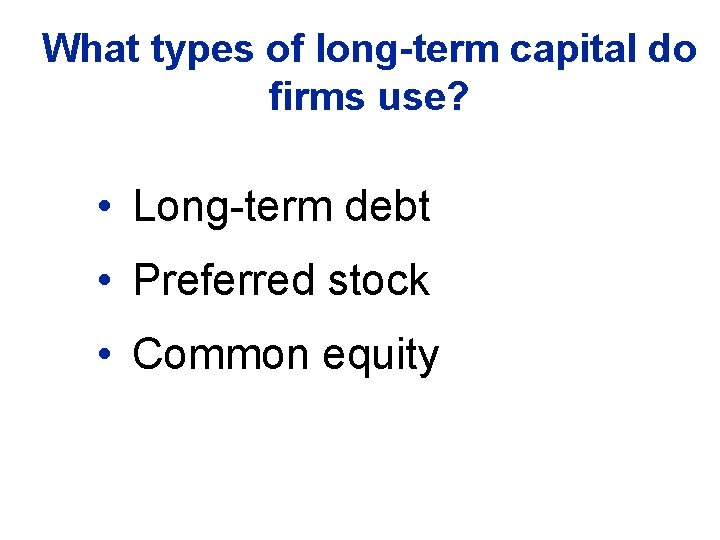
What types of long-term capital do firms use? • Long-term debt • Preferred stock • Common equity

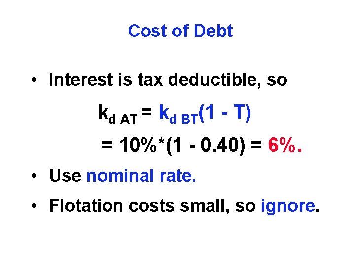
Cost of Debt • Interest is tax deductible, so kd AT = kd BT(1 - T) = 10%*(1 - 0. 40) = 6%. • Use nominal rate. • Flotation costs small, so ignore.

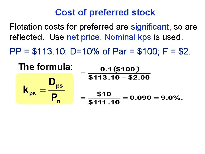
Cost of preferred stock Flotation costs for preferred are significant, so are reflected. Use net price. Nominal kps is used. PP = $113. 10; D=10% of Par = $100; F = $2. The formula:

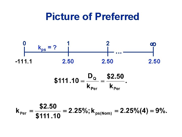
Picture of Preferred 0 -111. 1 kps = ? 1 2 2. 50 . . . 2. 50

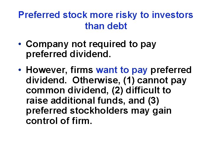
Preferred stock more risky to investors than debt • Company not required to pay preferred dividend. • However, firms want to pay preferred dividend. Otherwise, (1) cannot pay common dividend, (2) difficult to raise additional funds, and (3) preferred stockholders may gain control of firm.

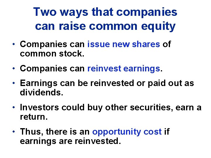
Two ways that companies can raise common equity • Companies can issue new shares of common stock. • Companies can reinvest earnings. • Earnings can be reinvested or paid out as dividends. • Investors could buy other securities, earn a return. • Thus, there is an opportunity cost if earnings are reinvested.

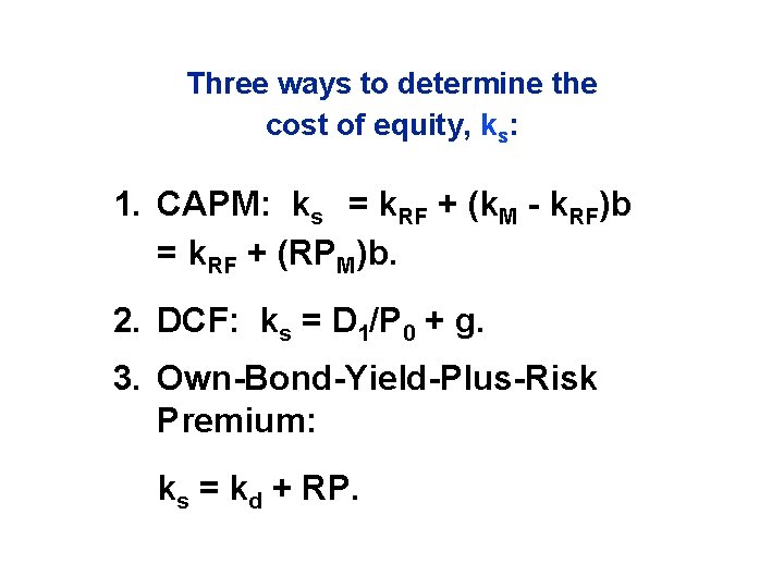
Three ways to determine the cost of equity, ks: 1. CAPM: ks = k. RF + (k. M - k. RF)b = k. RF + (RPM)b. 2. DCF: ks = D 1/P 0 + g. 3. Own-Bond-Yield-Plus-Risk Premium: ks = kd + RP.

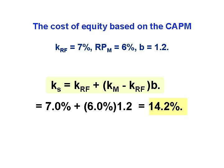
The cost of equity based on the CAPM k. RF = 7%, RPM = 6%, b = 1. 2. ks = k. RF + (k. M - k. RF )b. = 7. 0% + (6. 0%)1. 2 = 14. 2%.

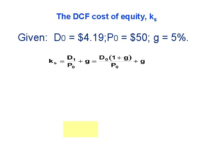
The DCF cost of equity, ks Given: D 0 = $4. 19; P 0 = $50; g = 5%.

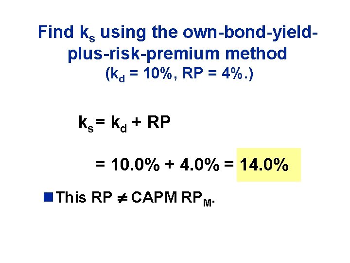
Find ks using the own-bond-yieldplus-risk-premium method (kd = 10%, RP = 4%. ) ks = kd + RP = 10. 0% + 4. 0% = 14. 0% n This RP CAPM RPM.

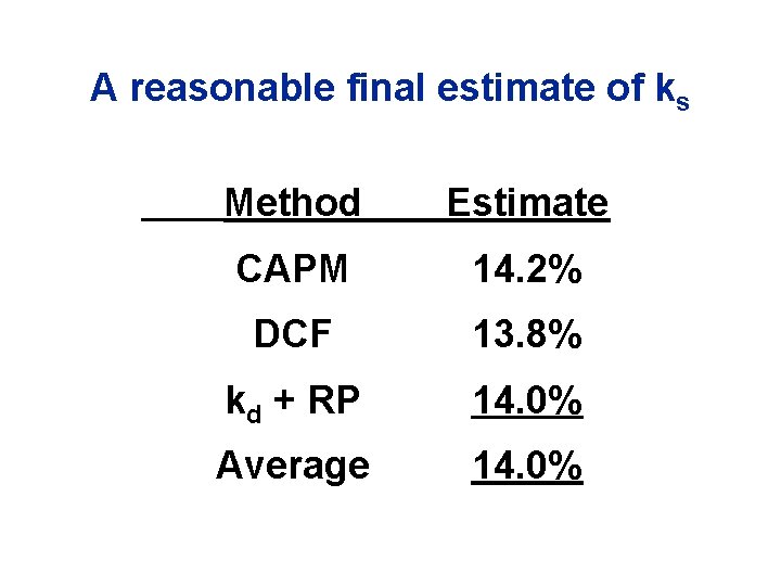
A reasonable final estimate of ks Method Estimate CAPM 14. 2% DCF 13. 8% kd + RP 14. 0% Average 14. 0%

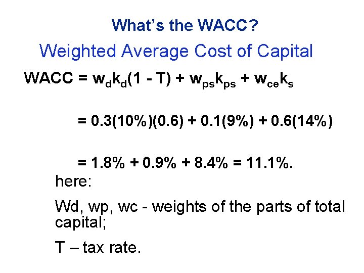
What’s the WACC? Weighted Average Cost of Capital WACC = wdkd(1 - T) + wpskps + wceks = 0. 3(10%)(0. 6) + 0. 1(9%) + 0. 6(14%) = 1. 8% + 0. 9% + 8. 4% = 11. 1%. here: Wd, wp, wc - weights of the parts of total capital; T – tax rate.

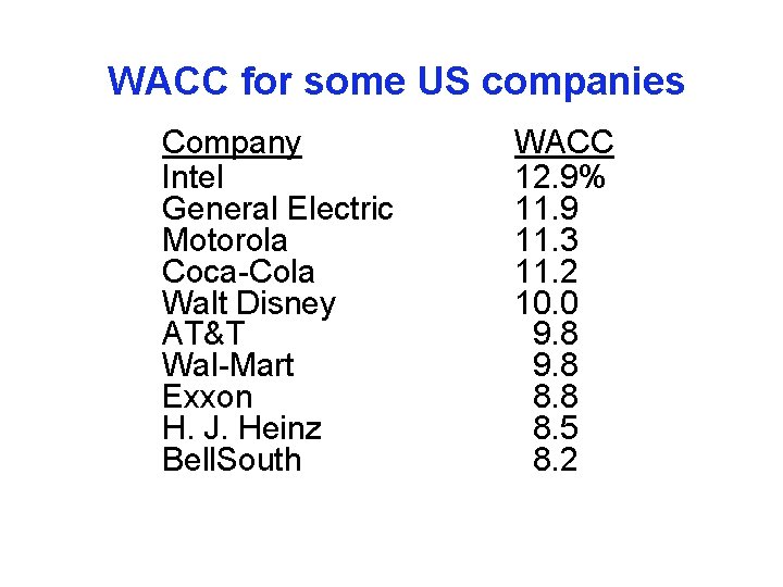
WACC for some US companies Company Intel General Electric Motorola Coca-Cola Walt Disney AT&T Wal-Mart Exxon H. J. Heinz Bell. South WACC 12. 9% 11. 9 11. 3 11. 2 10. 0 9. 8 8. 5 8. 2

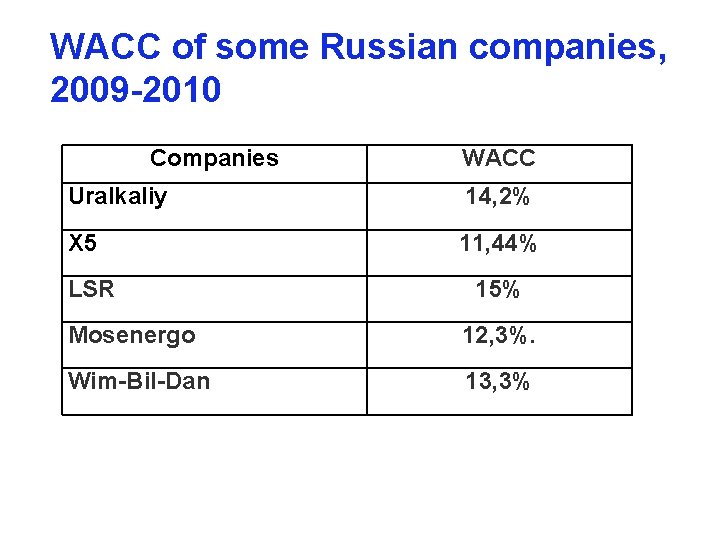
WACC of some Russian companies, 2009 -2010 Companies WACC Uralkaliy 14, 2% X 5 11, 44% LSR 15% Mosenergo 12, 3%. Wim-Bil-Dan 13, 3%

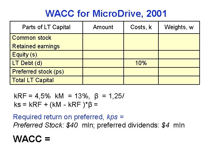
WACC for Micro. Drive, 2001 Parts of LT Capital Amount Common stock Retained earnings Equity (s) LT Debt (d) Preferred stock (ps) Total LT Capital Costs, k Weights, w 10% k. RF = 4, 5% k. M = 13%, β = 1, 25/ ks = k. RF + (k. M - k. RF )*β = Required return on preferred, kps = Preferred Stock: $40 mln; preferred dividends: $4 mln WACC =

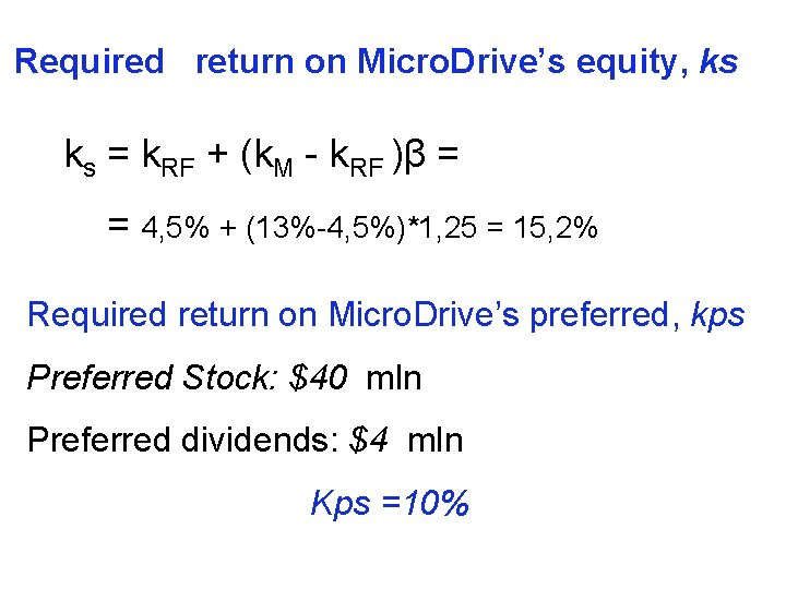
Required return on Micro. Drive’s equity, ks ks = k. RF + (k. M - k. RF )β = = 4, 5% + (13%-4, 5%)*1, 25 = 15, 2% Required return on Micro. Drive’s preferred, kps Preferred Stock: $40 mln Preferred dividends: $4 mln Kps =10%

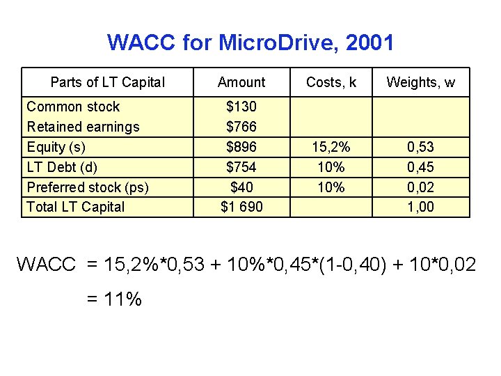
WACC for Micro. Drive, 2001 Parts of LT Capital Common stock Retained earnings Equity (s) LT Debt (d) Preferred stock (ps) Total LT Capital Amount Costs, k Weights, w $130 $766 $896 $754 $40 $1 690 15, 2% 10% 0, 53 0, 45 0, 02 1, 00 WACC = 15, 2%*0, 53 + 10%*0, 45*(1 -0, 40) + 10*0, 02 = 11%

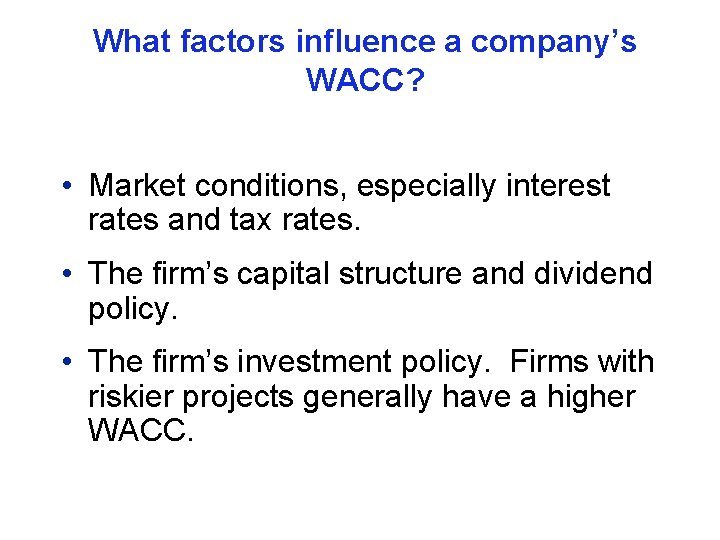
What factors influence a company’s WACC? • Market conditions, especially interest rates and tax rates. • The firm’s capital structure and dividend policy. • The firm’s investment policy. Firms with riskier projects generally have a higher WACC.

Should the company use the composite WACC as the hurdle rate for each of its projects? • NO! The composite WACC reflects the risk of an average project undertaken by the firm. Therefore, the WACC only represents the “hurdle rate” for a typical project with average risk. • Different projects have different risks. The project’s WACC should be adjusted to reflect the project’s risk.

6. Time Value of Money

Time Value of Money • Future value (FV) • Present value (PV) • Rates of return • Loan amortization Money (with similar nominal) paid or received at different points in time have different values (because of risks, alternative costs, and inflation).

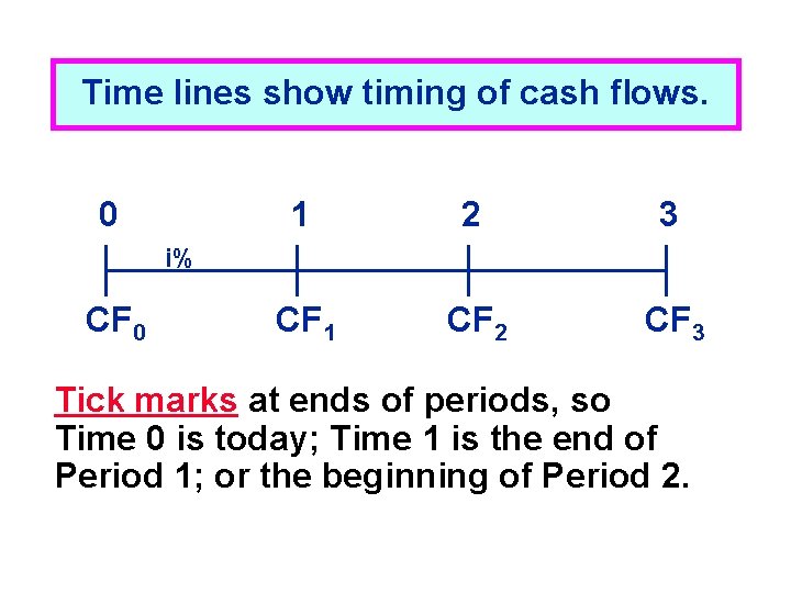
Time lines show timing of cash flows. 0 1 2 3 CF 1 CF 2 CF 3 i% CF 0 Tick marks at ends of periods, so Time 0 is today; Time 1 is the end of Period 1; or the beginning of Period 2.

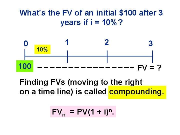
What’s the FV of an initial $100 after 3 years if i = 10%? 0 10% 1 2 100 3 FV = ? Finding FVs (moving to the right on a time line) is called compounding. FVn = PV(1 + i)n.

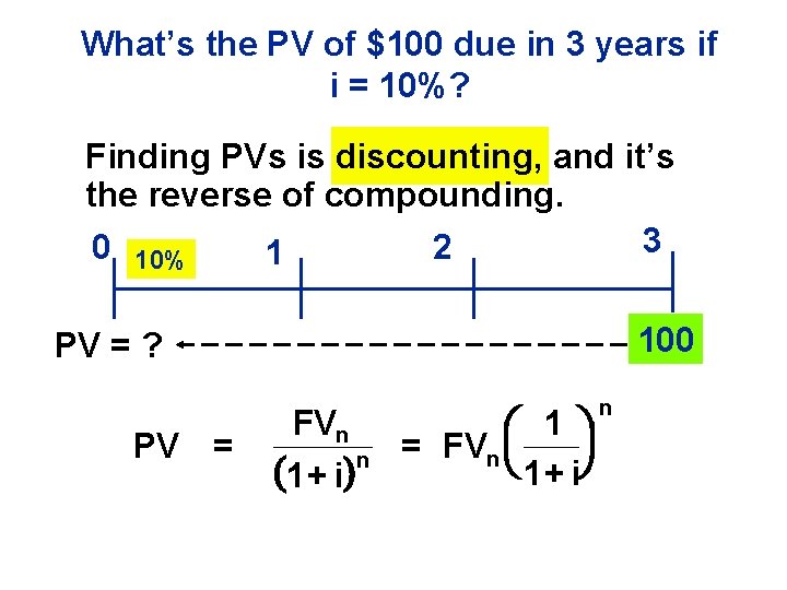
What’s the PV of $100 due in 3 years if i = 10%? Finding PVs is discounting, and it’s the reverse of compounding. 3 0 10% 2 1 100 PV = ? PV = FVn 1+ i n 1 = FVn 1+ i n

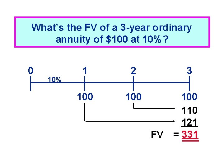
What’s the FV of a 3 -year ordinary annuity of $100 at 10%? 0 10% 1 2 100 3 100 110 121 FV = 331

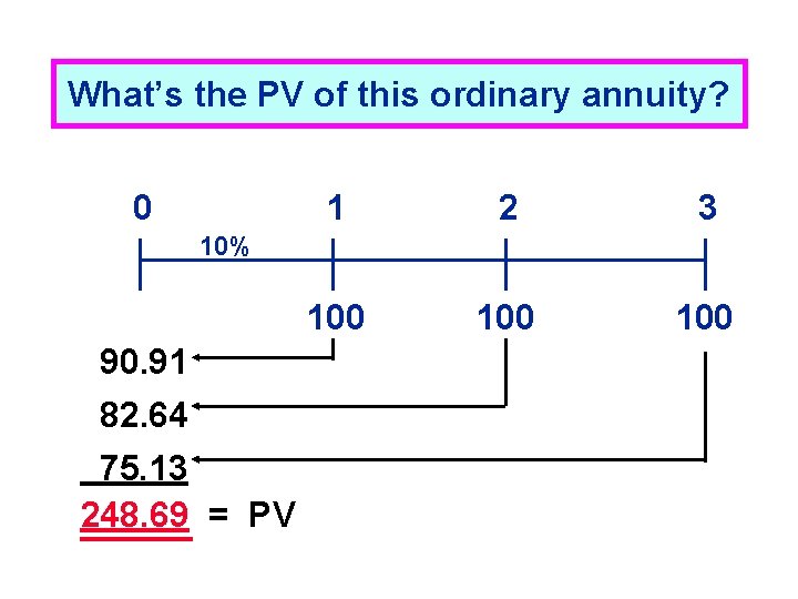
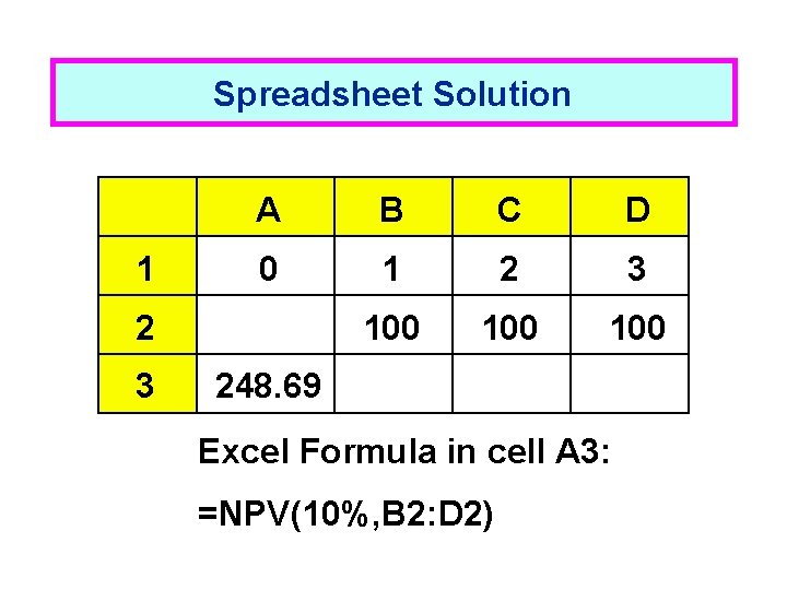
What’s the PV of this ordinary annuity? 0 1 2 3 100 100 10% 90. 91 82. 64 75. 13 248. 69 = PV

Spreadsheet Solution 1 A B C D 0 1 2 3 100 100 2 3 248. 69 Excel Formula in cell A 3: =NPV(10%, B 2: D 2)

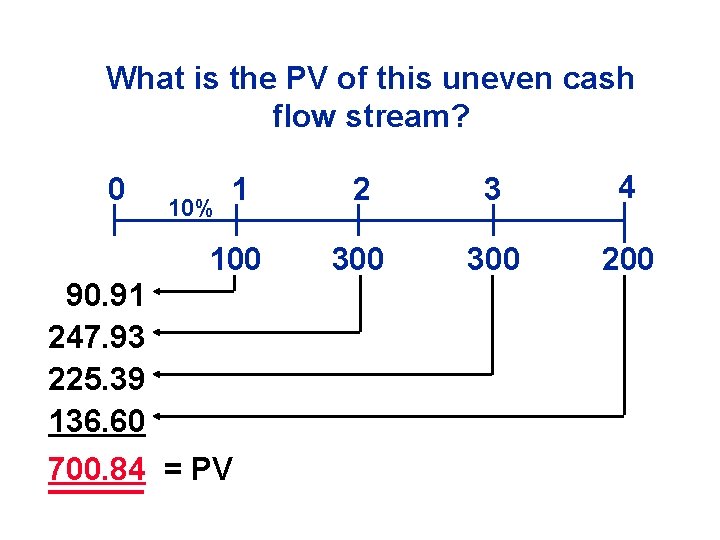
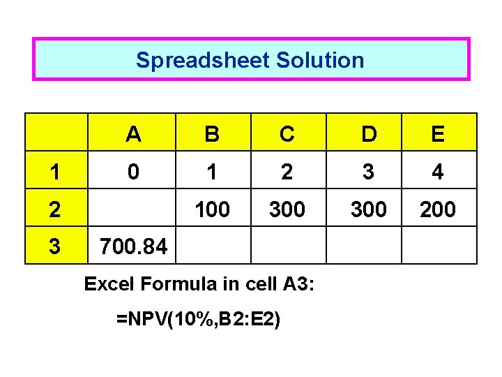
What is the PV of this uneven cash flow stream? 0 1 2 3 4 100 300 200 10% 90. 91 247. 93 225. 39 136. 60 700. 84 = PV

Spreadsheet Solution 1 A B C D E 0 1 2 3 4 100 300 2 3 700. 84 Excel Formula in cell A 3: =NPV(10%, B 2: E 2)

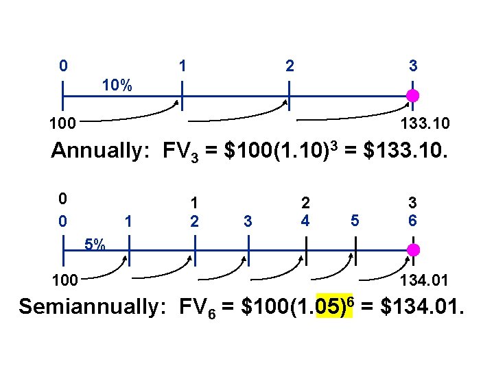
0 1 2 3 10% 100 133. 10 Annually: FV 3 = $100(1. 10)3 = $133. 10. 0 0 1 1 2 3 2 4 5 3 6 5% 100 134. 01 Semiannually: FV 6 = $100(1. 05)6 = $134. 01.

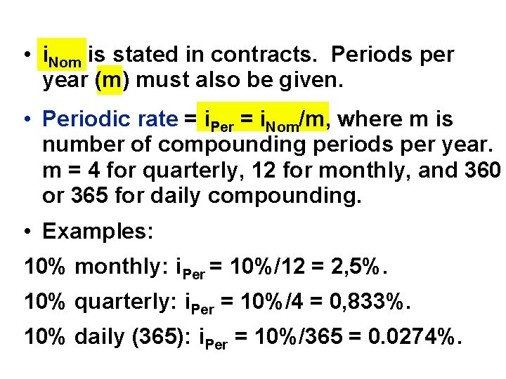
• i. Nom is stated in contracts. Periods per year (m) must also be given. • Periodic rate = i. Per = i. Nom/m, where m is number of compounding periods per year. m = 4 for quarterly, 12 for monthly, and 360 or 365 for daily compounding. • Examples: 10% monthly: i. Per = 10%/12 = 2, 5%. 10% quarterly: i. Per = 10%/4 = 0, 833%. 10% daily (365): i. Per = 10%/365 = 0. 0274%.

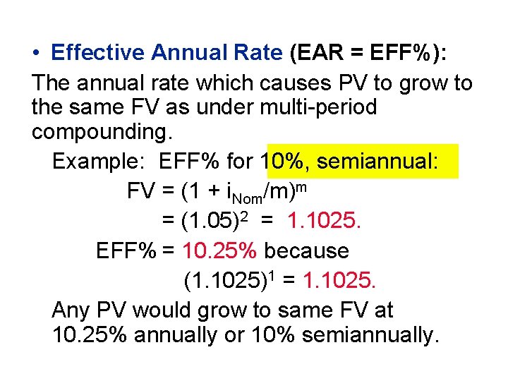
• Effective Annual Rate (EAR = EFF%): The annual rate which causes PV to grow to the same FV as under multi-period compounding. Example: EFF% for 10%, semiannual: FV = (1 + i. Nom/m)m = (1. 05)2 = 1. 1025. EFF% = 10. 25% because (1. 1025)1 = 1. 1025. Any PV would grow to same FV at 10. 25% annually or 10% semiannually.

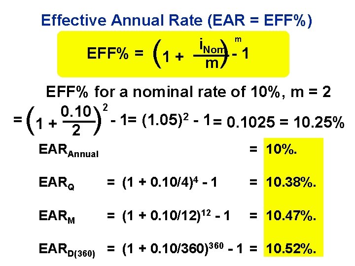
Effective Annual Rate (EAR = EFF%) EFF% = ( ) m i. Nom 1+ m -1 EFF% for a nominal rate of 10%, m = 2 0. 10 2 = 1+ - 1= (1. 05)2 - 1 = 0. 1025 = 10. 25% 2 ( ) EARAnnual = 10%. EARQ = (1 + 0. 10/4)4 - 1 = 10. 38%. EARM = (1 + 0. 10/12)12 - 1 = 10. 47%. EARD(360) = (1 + 0. 10/360)360 - 1 = 10. 52%.

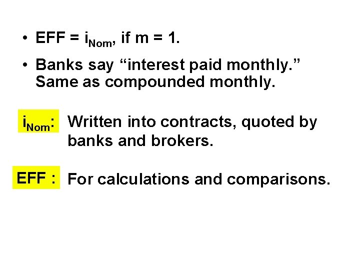
• EFF = i. Nom, if m = 1. • Banks say “interest paid monthly. ” Same as compounded monthly. i. Nom: Written into contracts, quoted by banks and brokers. EFF : For calculations and comparisons.

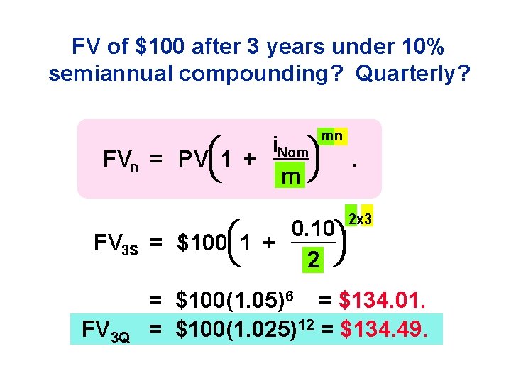
FV of $100 after 3 years under 10% semiannual compounding? Quarterly? i. Nom FVn = PV 1 + m FV 3 S FV 3 Q mn 0. 10 = $100 1 + 2 . 2 x 3 = $100(1. 05)6 = $134. 01. = $100(1. 025)12 = $134. 49.

Loan amortization table • A table that breaks down the periodic fixed payment of an installment loan into its principal and interest components. • The principal component of each payment reduces the remaining principal balance. • The interest component is the interest payment on the beginning-of-period principal balance. • Amortization tables are widely used-for home mortgages, auto loans, business loans, retirement plans, and so on.

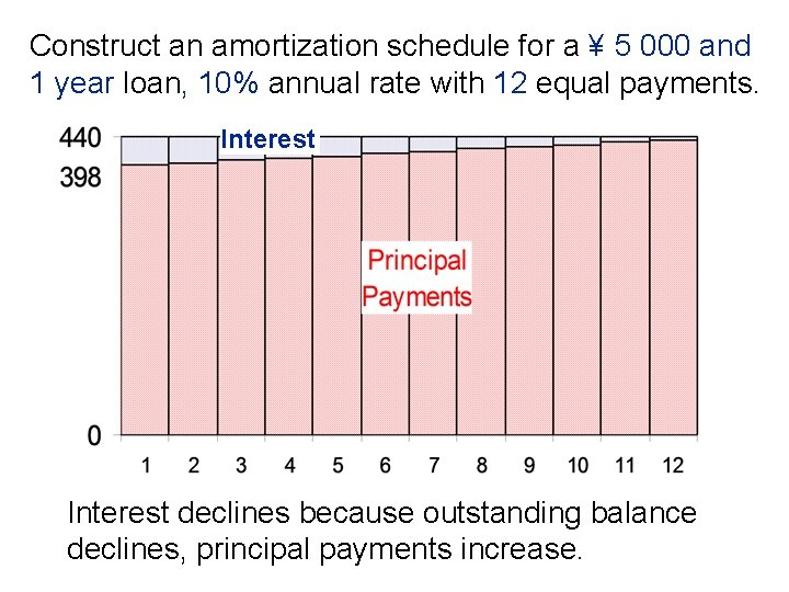
Construct an amortization schedule for a ¥ 5 000 and 1 year loan, 10% annual rate with 12 equal payments. Interest declines because outstanding balance declines, principal payments increase.

7. Basic Model of Capital Assets Valuation: Discounted Cash Flows. Bonds and Stocks Valuation.

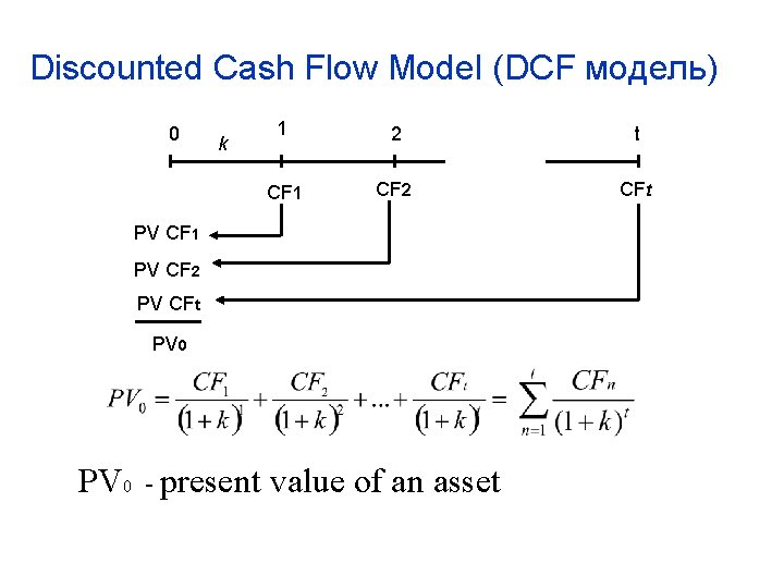
Discounted Cash Flow Model (DCF модель) 0 k 1 2 t CF 1 CF 2 CFt PV CF 1 PV CF 2 PV CFt PV 0 - present value of an asset

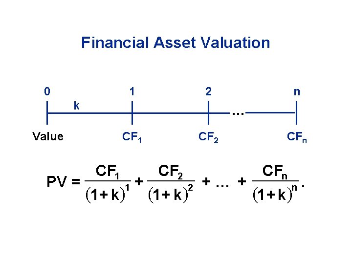
Financial Asset Valuation 0 1 2 k . . . Value PV = n CF 1 1+ k 1 + CF 2 1+ k 2 +. . . + CFn 1+ k n .

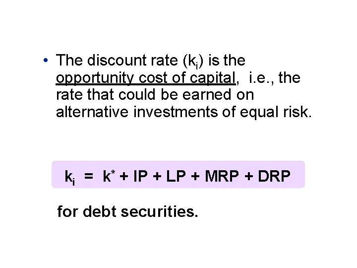
• The discount rate (ki) is the opportunity cost of capital, i. e. , the rate that could be earned on alternative investments of equal risk. ki = k* + IP + LP + MRP + DRP for debt securities.

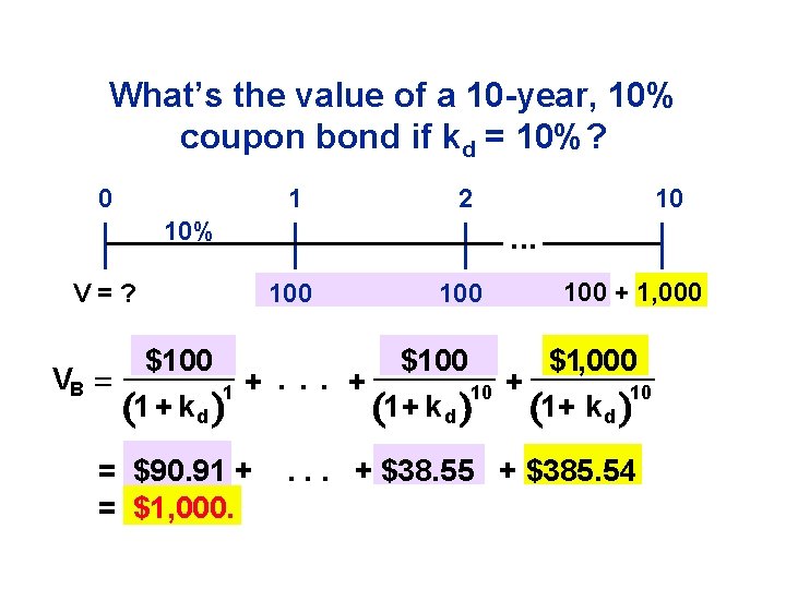
What’s the value of a 10 -year, 10% coupon bond if kd = 10%? 0 1 2 10% . . . V=? VB 10 100 $100 1 + k d 1 +. . . + = $90. 91 + = $1, 000. 100 + 1, 000 100 $100 1 + k d 10 + $1, 000 1+ k d 10 . . . + $38. 55 + $385. 54

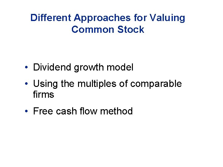
Different Approaches for Valuing Common Stock • Dividend growth model • Using the multiples of comparable firms • Free cash flow method

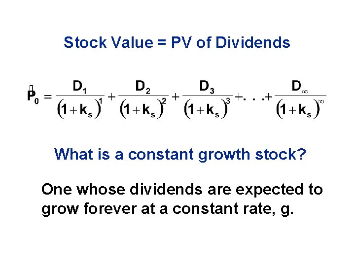
Stock Value = PV of Dividends What is a constant growth stock? One whose dividends are expected to grow forever at a constant rate, g.

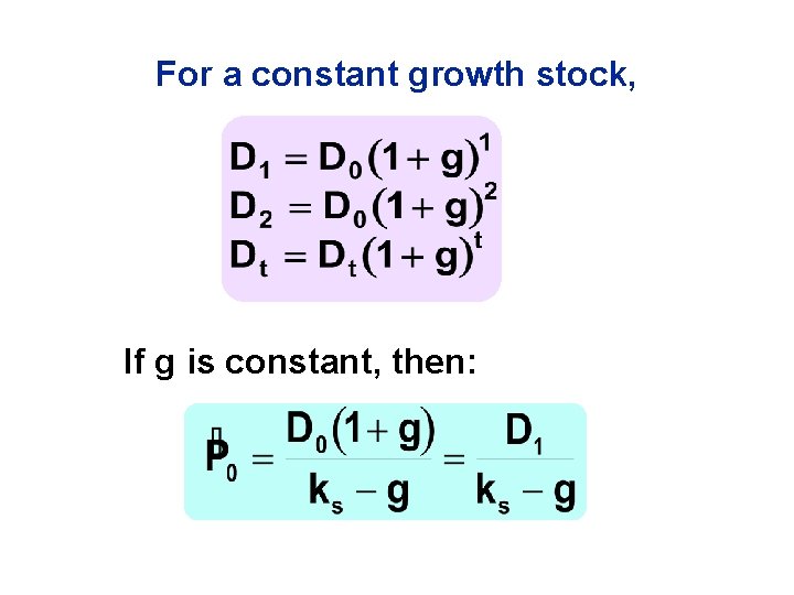
For a constant growth stock, If g is constant, then:

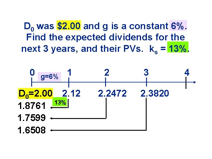
D 0 was $2. 00 and g is a constant 6%. Find the expected dividends for the next 3 years, and their PVs. ks = 13%. 0 g=6% 1 D 0=2. 00 2. 12 13% 1. 8761 1. 7599 1. 6508 2 2. 2472 3 2. 3820 4

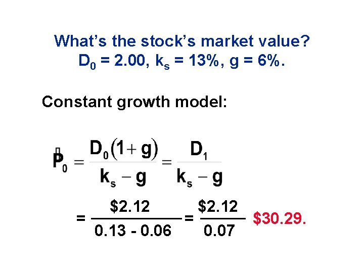
What’s the stock’s market value? D 0 = 2. 00, ks = 13%, g = 6%. Constant growth model: $2. 12 = = $30. 29. 0. 13 - 0. 06 0. 07

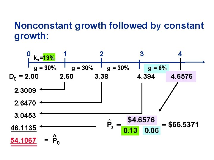
Nonconstant growth followed by constant growth: 0 k =13% s 1 g = 30% D 0 = 2. 00 g = 30% 2. 60 2. 3009 2. 6470 3. 0453 46. 1135 54. 1067 2 ^ = P 0 3 g = 30% 3. 38 4 g = 6% 4. 394 4. 6576

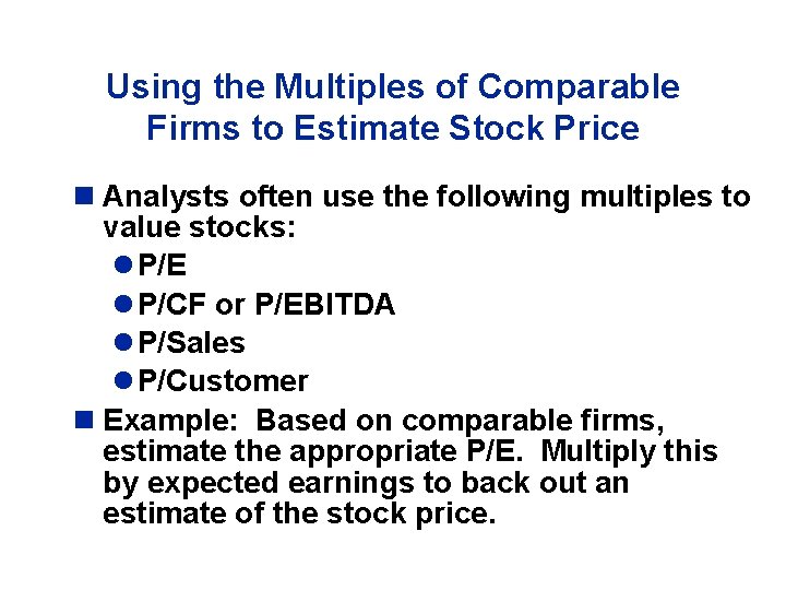
Using the Multiples of Comparable Firms to Estimate Stock Price n Analysts often use the following multiples to value stocks: l P/E l P/CF or P/EBITDA l P/Sales l P/Customer n Example: Based on comparable firms, estimate the appropriate P/E. Multiply this by expected earnings to back out an estimate of the stock price.