FIN 30220 Macroeconomics Using Economic Data There are

FIN 30220: Macroeconomics Using Economic Data

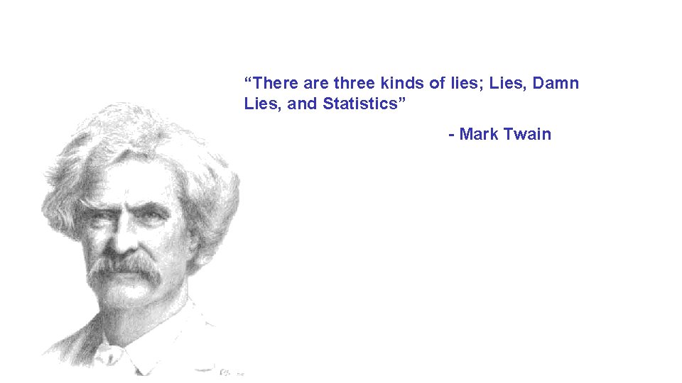
“There are three kinds of lies; Lies, Damn Lies, and Statistics” - Mark Twain

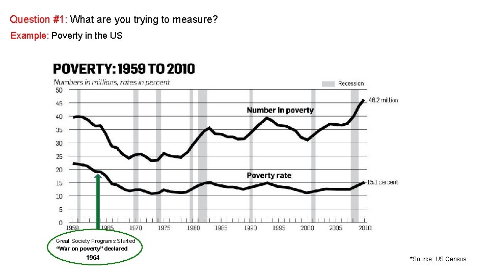
Question #1: What are you trying to measure? Example: Poverty in the US Great Society Programs Started “War on poverty” declared 1964 *Source: US Census

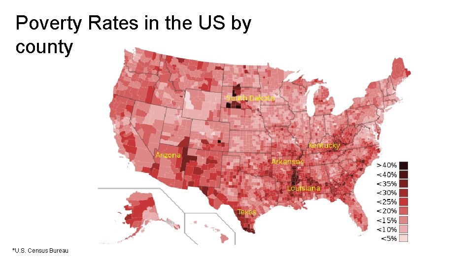
Poverty Rates in the US by county *U. S. Census Bureau

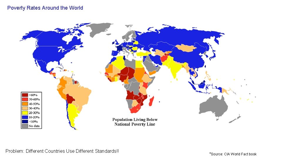
Poverty Rates Around the World Problem: Different Countries Use Different Standards!! *Source: CIA World Fact book

e w o d ? y w t o r e H v o p e n i f e d

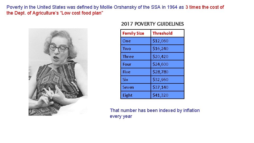
Poverty in the United States was defined by Mollie Orshansky of the SSA in 1964 as 3 times the cost of the Dept. of Agriculture’s “Low cost food plan” 2017 POVERTY GUIDELINES Family Size Threshold One $12, 060 Two $16, 240 Three $20, 420 Four $24, 600 Five $28, 780 Six $32, 960 Seven $37, 140 Eight $41, 320 That number has been indexed by inflation every year

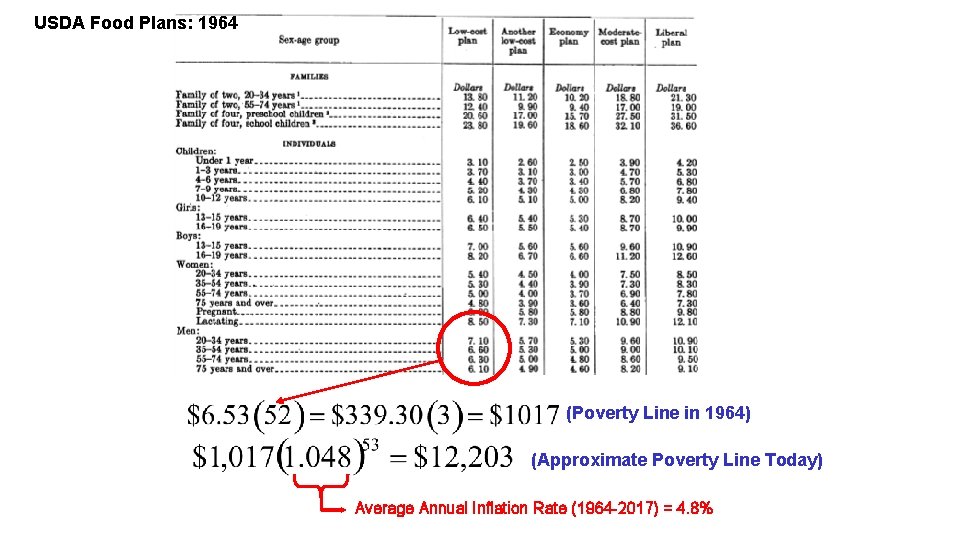
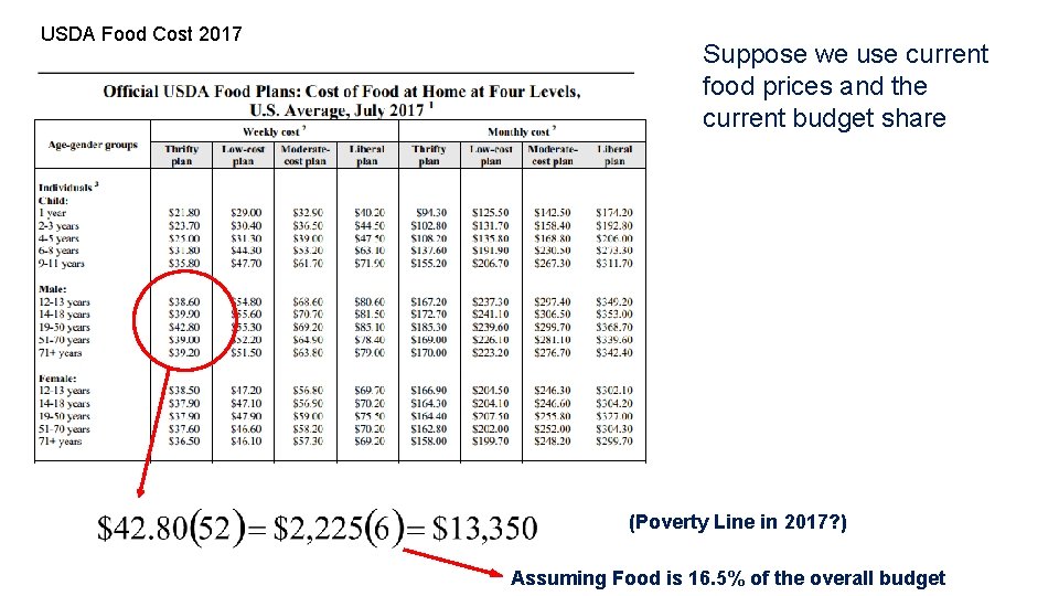
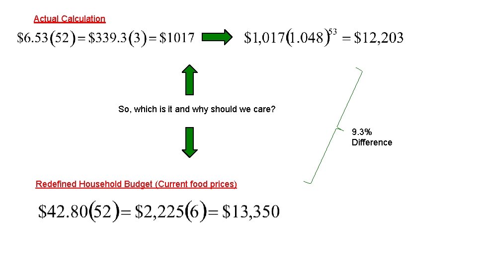
USDA Food Plans: 1964 (Poverty Line in 1964) (Approximate Poverty Line Today) Average Annual Inflation Rate (1964 -2017) = 4. 8%

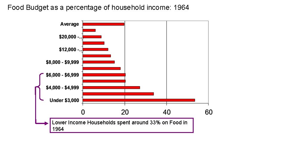
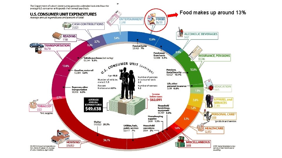
Food Budget as a percentage of household income: 1964 Lower Income Households spent around 33% on Food in 1964

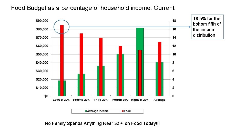
Food Budget as a percentage of household income: Current 16. 5% for the bottom fifth of the income distribution No Family Spends Anything Near 33% on Food Today!!!

Food makes up around 13%

USDA Food Cost 2017 Suppose we use current food prices and the current budget share (Poverty Line in 2017? ) Assuming Food is 16. 5% of the overall budget

Actual Calculation So, which is it and why should we care? 9. 3% Difference Redefined Household Budget (Current food prices)

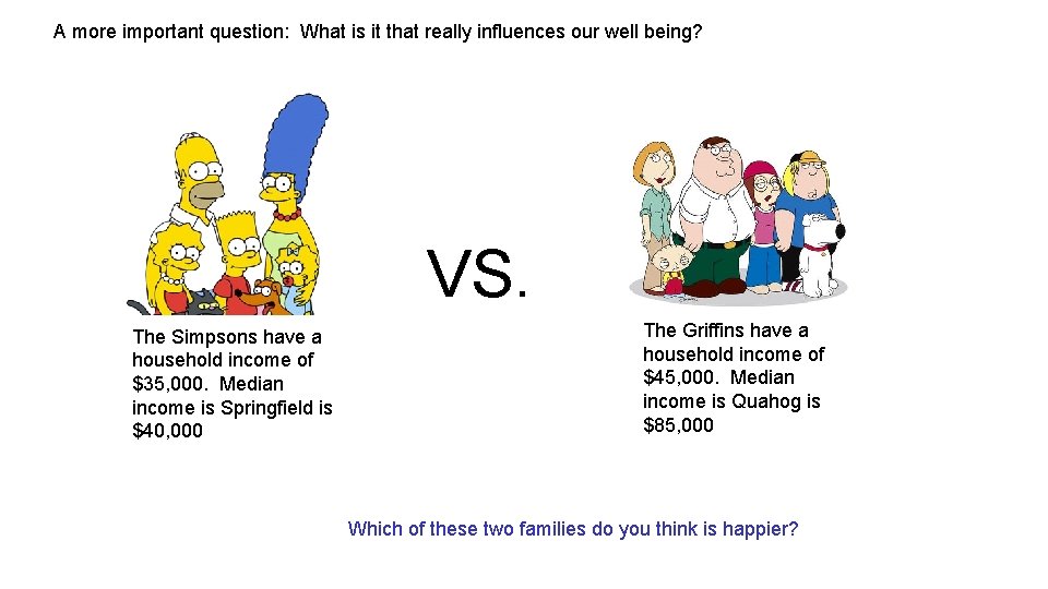
A more important question: What is it that really influences our well being? VS. The Simpsons have a household income of $35, 000. Median income is Springfield is $40, 000 The Griffins have a household income of $45, 000. Median income is Quahog is $85, 000 Which of these two families do you think is happier?

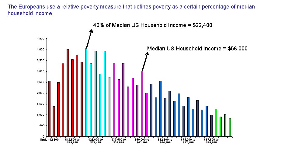
The Europeans use a relative poverty measure that defines poverty as a certain percentage of median household income 40% of Median US Household Income = $22, 400 Median US Household Income = $56, 000

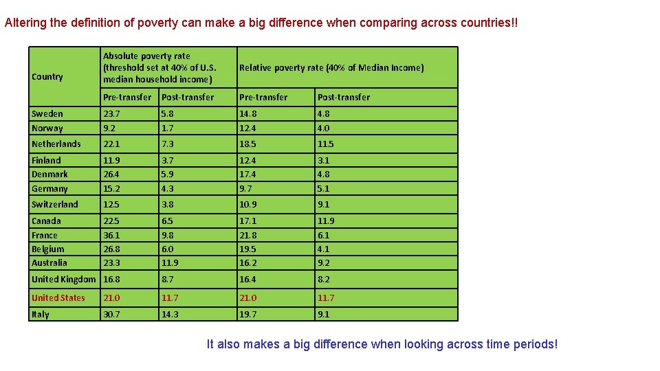
Altering the definition of poverty can make a big difference when comparing across countries!! Absolute poverty rate (threshold set at 40% of U. S. median household income) Relative poverty rate (40% of Median Income) Pre-transfer Post-transfer Sweden Norway 23. 7 9. 2 5. 8 1. 7 14. 8 12. 4 4. 8 4. 0 Netherlands 22. 1 7. 3 18. 5 11. 5 Finland Denmark Germany 11. 9 26. 4 15. 2 3. 7 5. 9 4. 3 12. 4 17. 4 9. 7 3. 1 4. 8 5. 1 Switzerland 12. 5 3. 8 10. 9 9. 1 Canada France Belgium Australia 22. 5 36. 1 26. 8 23. 3 6. 5 9. 8 6. 0 11. 9 17. 1 21. 8 19. 5 16. 2 11. 9 6. 1 4. 1 9. 2 United Kingdom 16. 8 8. 7 16. 4 8. 2 United States 21. 0 11. 7 Italy 30. 7 14. 3 19. 7 9. 1 Country It also makes a big difference when looking across time periods!

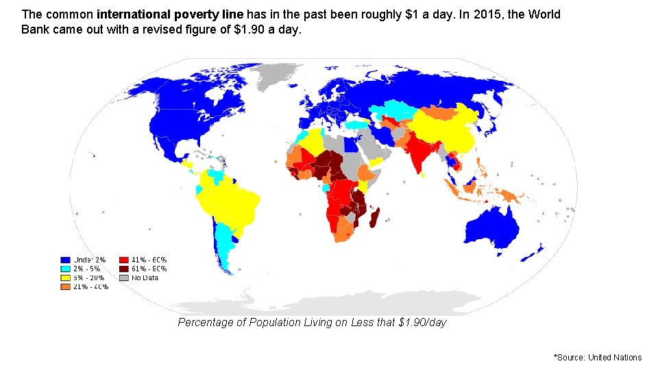
The common international poverty line has in the past been roughly $1 a day. In 2015, the World Bank came out with a revised figure of $1. 90 a day. Percentage of Population Living on Less that $1. 90/day *Source: United Nations

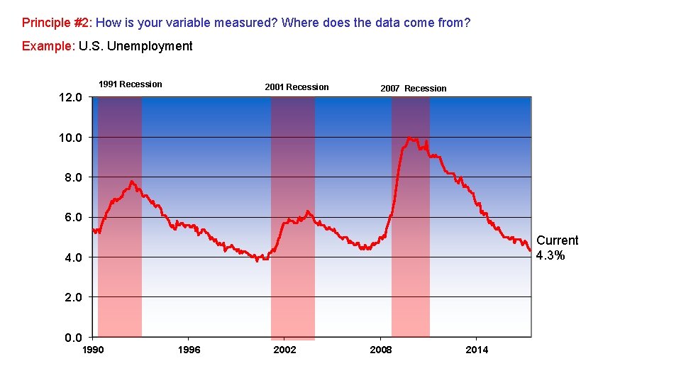
Principle #2: How is your variable measured? Where does the data come from? Example: U. S. Unemployment 1991 Recession 2001 Recession 12. 0 2007 Recession 10. 0 8. 0 6. 0 Current 4. 3% 4. 0 2. 0 0. 0 1996 2002 2008 2014

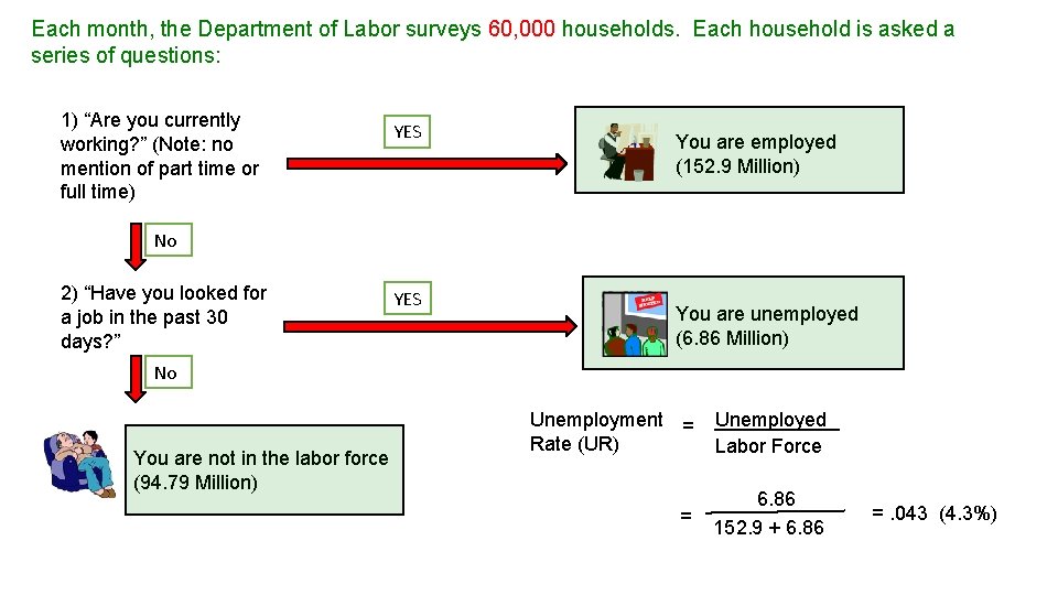
Each month, the Department of Labor surveys 60, 000 households. Each household is asked a series of questions: 1) “Are you currently working? ” (Note: no mention of part time or full time) YES You are employed (152. 9 Million) No 2) “Have you looked for a job in the past 30 days? ” YES You are unemployed (6. 86 Million) No You are not in the labor force (94. 79 Million) Unemployment = Rate (UR) Unemployed Labor Force = 6. 86 152. 9 + 6. 86 =. 043 (4. 3%)

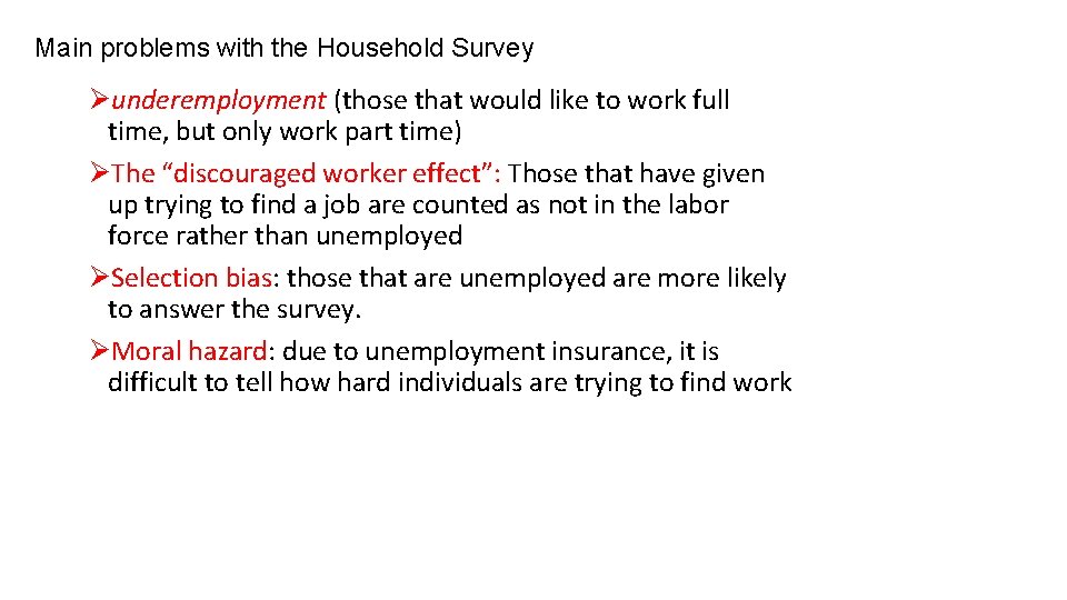
Main problems with the Household Survey Øunderemployment (those that would like to work full time, but only work part time) ØThe “discouraged worker effect”: Those that have given up trying to find a job are counted as not in the labor force rather than unemployed ØSelection bias: those that are unemployed are more likely to answer the survey. ØMoral hazard: due to unemployment insurance, it is difficult to tell how hard individuals are trying to find work

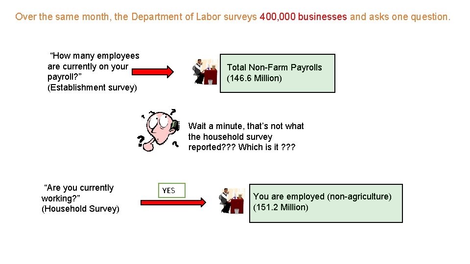
Over the same month, the Department of Labor surveys 400, 000 businesses and asks one question. “How many employees are currently on your payroll? ” (Establishment survey) Total Non-Farm Payrolls (146. 6 Million) Wait a minute, that’s not what the household survey reported? ? ? Which is it ? ? ? “Are you currently working? ” (Household Survey) YES You are employed (non-agriculture) (151. 2 Million)

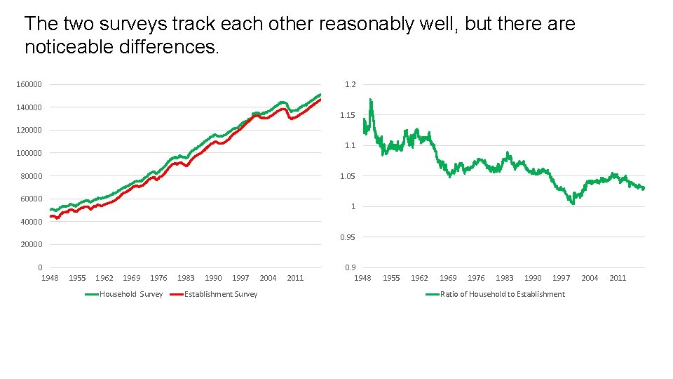
The two surveys track each other reasonably well, but there are noticeable differences. 160000 1. 2 140000 1. 15 120000 1. 1 100000 80000 1. 05 60000 1 40000 0. 95 20000 0 1948 1955 1962 1969 1976 Household Survey 1983 1990 1997 Establishment Survey 2004 2011 0. 9 1948 1955 1962 1969 1976 1983 1990 1997 Ratio of Household to Establishment 2004 2011

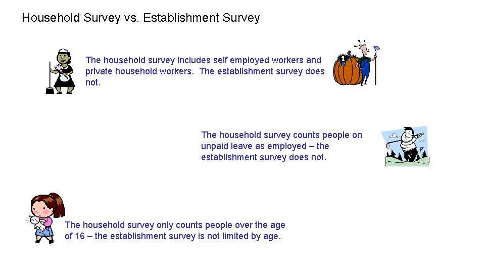
Household Survey vs. Establishment Survey The household survey includes self employed workers and private household workers. The establishment survey does not. The household survey counts people on unpaid leave as employed – the establishment survey does not. The household survey only counts people over the age of 16 – the establishment survey is not limited by age.

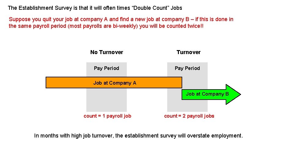
The Establishment Survey is that it will often times “Double Count” Jobs Suppose you quit your job at company A and find a new job at company B – if this is done in the same payroll period (most payrolls are bi-weekly) you will be counted twice!! No Turnover Pay Period Job at Company A Job at Company B count = 1 payroll job count = 2 payroll jobs In months with high job turnover, the establishment survey will overstate employment.

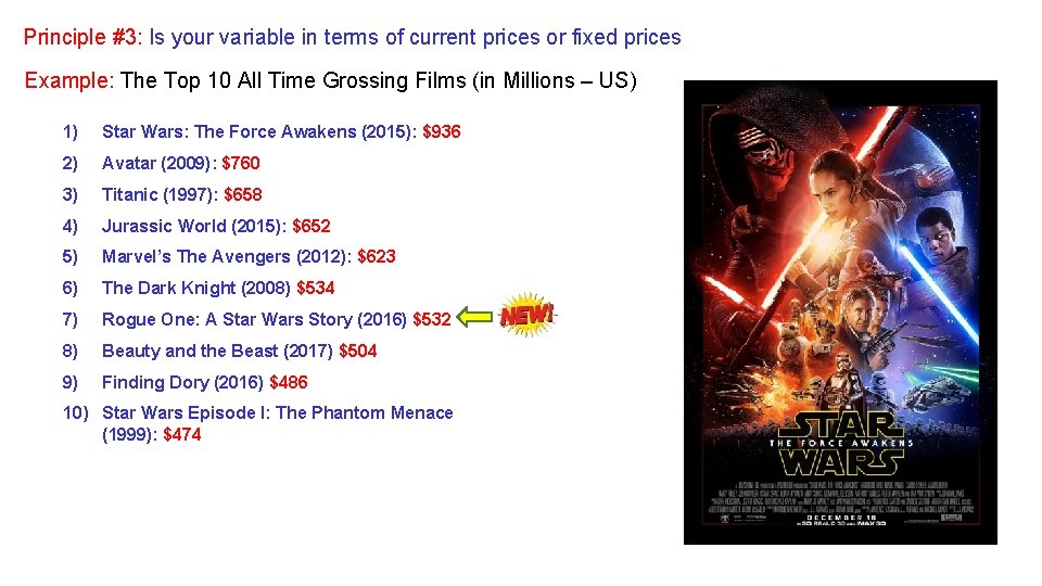
Principle #3: Is your variable in terms of current prices or fixed prices Example: The Top 10 All Time Grossing Films (in Millions – US) 1) Star Wars: The Force Awakens (2015): $936 2) Avatar (2009): $760 3) Titanic (1997): $658 4) Jurassic World (2015): $652 5) Marvel’s The Avengers (2012): $623 6) The Dark Knight (2008) $534 7) Rogue One: A Star Wars Story (2016) $532 8) Beauty and the Beast (2017) $504 9) Finding Dory (2016) $486 10) Star Wars Episode I: The Phantom Menace (1999): $474

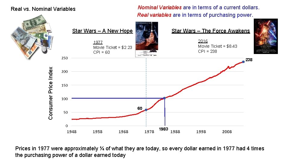
Nominal Variables are in terms of a current dollars. Real variables are in terms of purchasing power. Real vs. Nominal Variables Star Wars – The Force Awakens Star Wars – A New Hope 2016 Movie Ticket = $8. 43 CPI = 238 1977 Movie Ticket = $2. 23 CPI = 60 Consumer Price Index 250 238 200 150 100 60 50 0 1948 1958 1968 1978 1983 1988 1998 2008 Prices in 1977 were approximately ¼ of what they are today, so every dollar earned in 1977 had 4 times the purchasing power of a dollar earned today

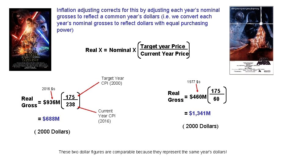
Inflation adjusting corrects for this by adjusting each year’s nominal grosses to reflect a common year’s dollars (i. e. we convert each year’s nominal grosses to reflect dollars with equal purchasing power) Real X = Nominal X Target Year CPI (2000) 2016 $s Real = $936 M Gross ( 2000 Dollars) 1977 $s 175 Real = $460 M 60 Gross 175 238 = $688 M Target year Price Current Year CPI (2016) = $1, 341 M ( 2000 Dollars) These two dollar figures are comparable because they represent the same year’s dollars!

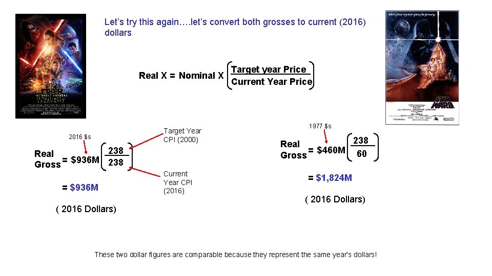
Let’s try this again…. let’s convert both grosses to current (2016) dollars Real X = Nominal X Target Year CPI (2000) 2016 $s 238 Real = $936 M 238 Gross = $936 M ( 2016 Dollars) Current Year CPI (2016) Target year Price Current Year Price 1977 $s 238 Real = $460 M 60 Gross = $1, 824 M ( 2016 Dollars) These two dollar figures are comparable because they represent the same year’s dollars!

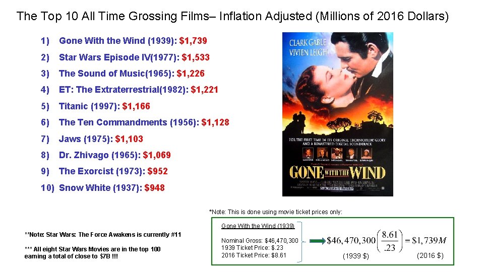
The Top 10 All Time Grossing Films– Inflation Adjusted (Millions of 2016 Dollars) 1) Gone With the Wind (1939): $1, 739 2) Star Wars Episode IV(1977): $1, 533 3) The Sound of Music(1965): $1, 226 4) ET: The Extraterrestrial(1982): $1, 221 5) Titanic (1997): $1, 166 6) The Ten Commandments (1956): $1, 128 7) Jaws (1975): $1, 103 8) Dr. Zhivago (1965): $1, 069 9) The Exorcist (1973): $952 10) Snow White (1937): $948 *Note: This is done using movie ticket prices only: Gone With the Wind (1939) **Note: Star Wars: The Force Awakens is currently #11 *** All eight Star Wars Movies are in the top 100 earning a total of close to $7 B !!! Nominal Gross: $46, 470, 300 1939 Ticket Price: $. 23 2016 Ticket Price: $8. 61 (1939 $) (2016 $)

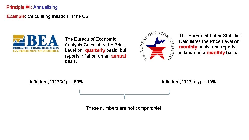
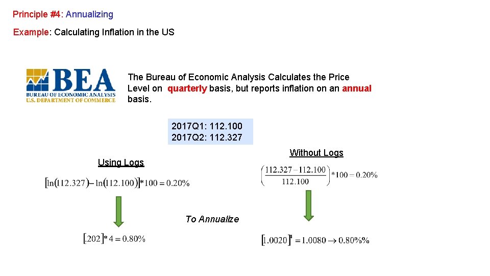
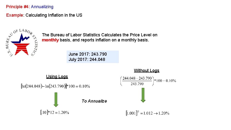
Principle #4: Annualizing Example: Calculating Inflation in the US The Bureau of Economic Analysis Calculates the Price Level on quarterly basis, but reports inflation on an annual basis. Inflation (2017 Q 2) =. 80% The Bureau of Labor Statistics Calculates the Price Level on monthly basis, and reports inflation on a monthly basis. Inflation (2017 July) =. 10% These numbers are not comparable!

Principle #4: Annualizing Example: Calculating Inflation in the US The Bureau of Economic Analysis Calculates the Price Level on quarterly basis, but reports inflation on an annual basis. 2017 Q 1: 112. 100 2017 Q 2: 112. 327 Without Logs Using Logs To Annualize

Principle #4: Annualizing Example: Calculating Inflation in the US The Bureau of Labor Statistics Calculates the Price Level on monthly basis, and reports inflation on a monthly basis. June 2017: 243. 790 July 2017: 244. 048 Without Logs Using Logs To Annualize

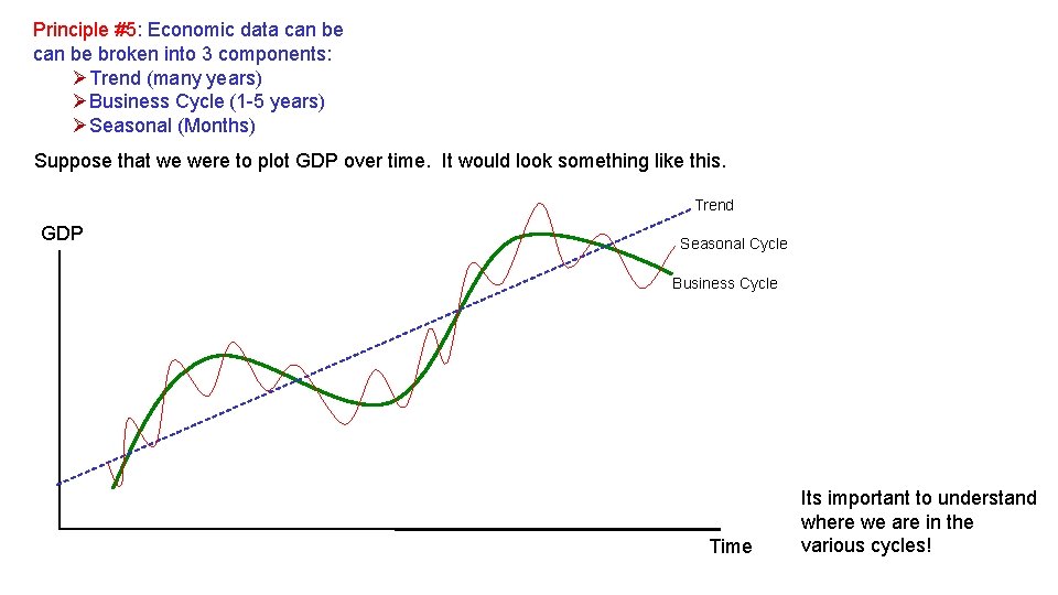
Principle #5: Economic data can be broken into 3 components: ØTrend (many years) ØBusiness Cycle (1 -5 years) ØSeasonal (Months) Suppose that we were to plot GDP over time. It would look something like this. Trend GDP Seasonal Cycle Business Cycle Time Its important to understand where we are in the various cycles!

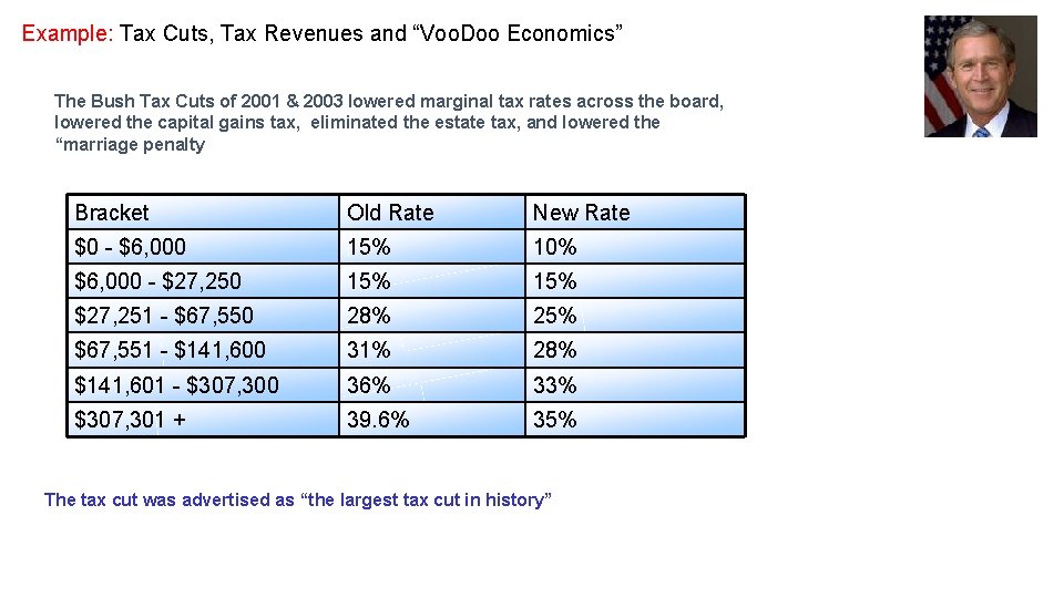
Example: Tax Cuts, Tax Revenues and “Voo. Doo Economics” The Bush Tax Cuts of 2001 & 2003 lowered marginal tax rates across the board, lowered the capital gains tax, eliminated the estate tax, and lowered the “marriage penalty Bracket Old Rate New Rate $0 - $6, 000 15% 10% $6, 000 - $27, 250 15% $27, 251 - $67, 550 28% 25% $67, 551 - $141, 600 31% 28% $141, 601 - $307, 300 36% 33% $307, 301 + 39. 6% 35% The tax cut was advertised as “the largest tax cut in history”

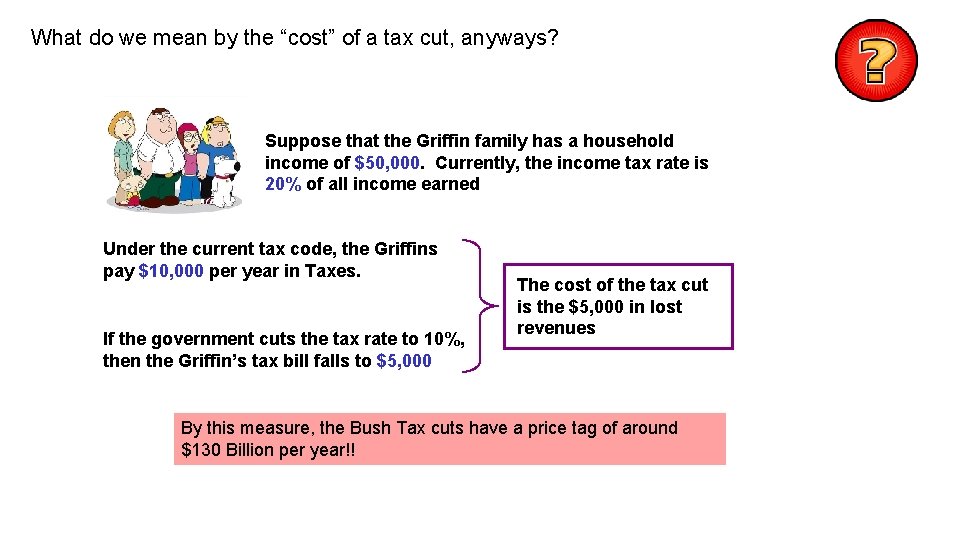
What do we mean by the “cost” of a tax cut, anyways? Suppose that the Griffin family has a household income of $50, 000. Currently, the income tax rate is 20% of all income earned Under the current tax code, the Griffins pay $10, 000 per year in Taxes. If the government cuts the tax rate to 10%, then the Griffin’s tax bill falls to $5, 000 The cost of the tax cut is the $5, 000 in lost revenues By this measure, the Bush Tax cuts have a price tag of around $130 Billion per year!!

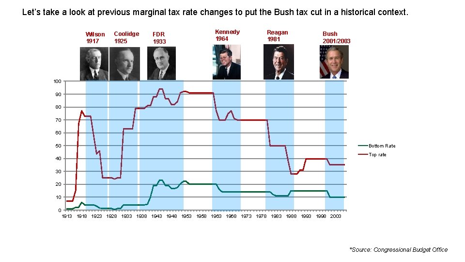
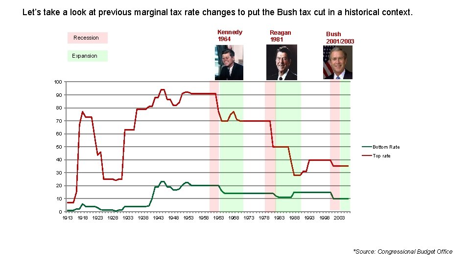
Let’s take a look at previous marginal tax rate changes to put the Bush tax cut in a historical context. Wilson 1917 Coolidge 1925 FDR 1933 Kennedy 1964 Reagan 1981 Bush 2001/2003 100 90 80 70 60 Bottom Rate 50 Top rate 40 30 20 10 0 1913 1918 1923 1928 1933 1938 1943 1948 1953 1958 1963 1968 1973 1978 1983 1988 1993 1998 2003 *Source: Congressional Budget Office

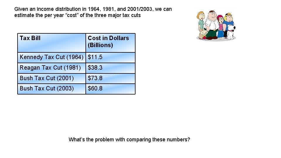
Given an income distribution in 1964, 1981, and 2001/2003, we can estimate the per year “cost” of the three major tax cuts Tax Bill Cost in Dollars (Billions) Kennedy Tax Cut (1964) $11. 5 Reagan Tax Cut (1981) $38. 3 Bush Tax Cut (2001) $73. 8 Bush Tax Cut (2003) $60. 8 What’s the problem with comparing these numbers?

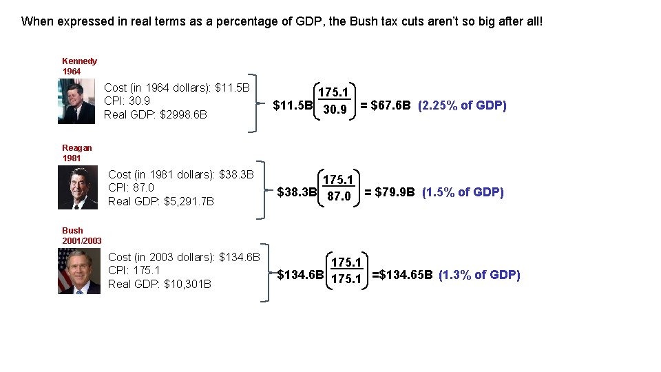
When expressed in real terms as a percentage of GDP, the Bush tax cuts aren’t so big after all! Kennedy 1964 Cost (in 1964 dollars): $11. 5 B CPI: 30. 9 Real GDP: $2998. 6 B 175. 1 $11. 5 B 30. 9 = $67. 6 B (2. 25% of GDP) Reagan 1981 Cost (in 1981 dollars): $38. 3 B CPI: 87. 0 Real GDP: $5, 291. 7 B 175. 1 $38. 3 B 87. 0 = $79. 9 B (1. 5% of GDP) Cost (in 2003 dollars): $134. 6 B CPI: 175. 1 Real GDP: $10, 301 B 175. 1 $134. 6 B 175. 1 =$134. 65 B (1. 3% of GDP) Bush 2001/2003

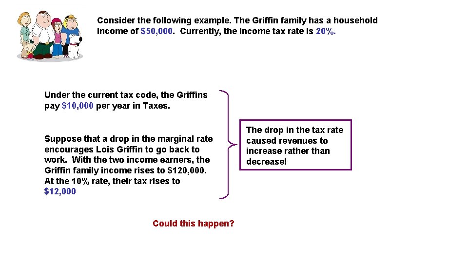
Consider the following example. The Griffin family has a household income of $50, 000. Currently, the income tax rate is 20%. Under the current tax code, the Griffins pay $10, 000 per year in Taxes. Suppose that a drop in the marginal rate encourages Lois Griffin to go back to work. With the two income earners, the Griffin family income rises to $120, 000. At the 10% rate, their tax rises to $12, 000 Could this happen? The drop in the tax rate caused revenues to increase rather than decrease!

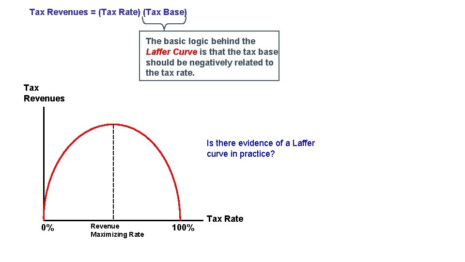
Tax Revenues = (Tax Rate) (Tax Base) The basic logic behind the Laffer Curve is that the tax base should be negatively related to the tax rate. Tax Revenues Is there evidence of a Laffer curve in practice? 0% Revenue Maximizing Rate 100% Tax Rate

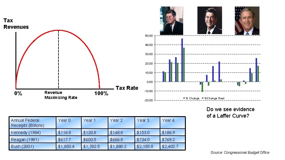
Tax Revenues 50. 00 40. 00 30. 00 20. 00 10. 00 0% Revenue Maximizing Rate 100% Tax Rate -10. 00 % Change -20. 00 Annual Federal Receipts (Billions) Year 0 Year 1 Year 2 Year 3 Year 4 Kennedy (1964) $116. 8 $130. 8 $148. 8 $153. 0 $186. 9 Reagan (1981) $617. 7 $600. 5 $666. 5 $734. 0 $769. 2 Bush (2001) $1, 853. 4 $1, 782. 5 $1, 880. 2 $2, 153. 8 $2, 402. 7 %Change Real Do we see evidence of a Laffer Curve? Source: Congressional Budget Office

Let’s take a look at previous marginal tax rate changes to put the Bush tax cut in a historical context. Recession Kennedy 1964 Reagan 1981 Bush 2001/2003 Expansion 100 90 80 70 60 Bottom Rate 50 Top rate 40 30 20 10 0 1913 1918 1923 1928 1933 1938 1943 1948 1953 1958 1963 1968 1973 1978 1983 1988 1993 1998 2003 *Source: Congressional Budget Office

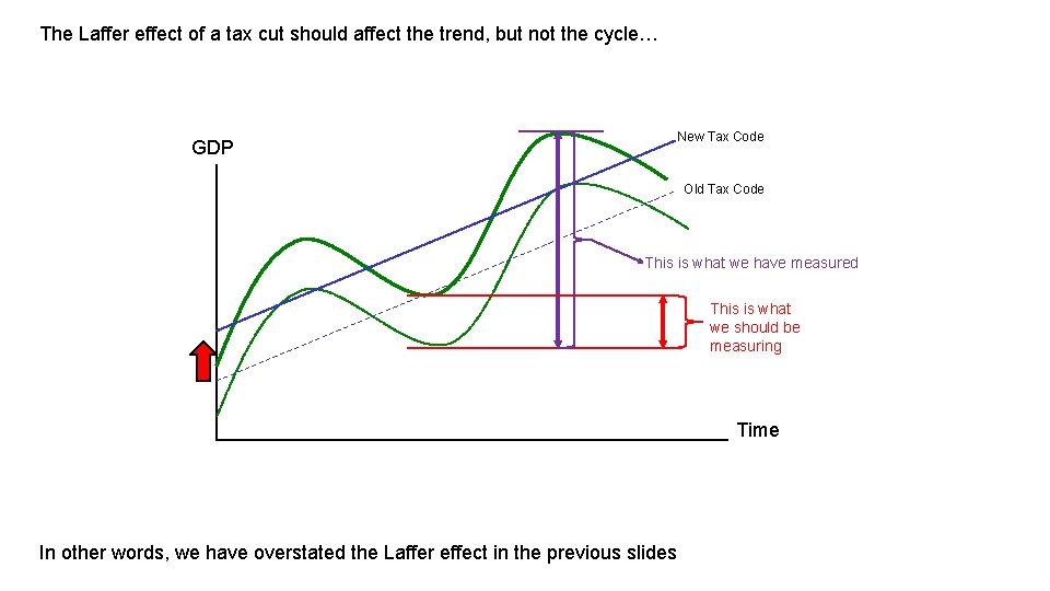
The Laffer effect of a tax cut should affect the trend, but not the cycle… New Tax Code GDP Old Tax Code This is what we have measured This is what we should be measuring Time In other words, we have overstated the Laffer effect in the previous slides