Filtering in the Spatial Domain Filtering the spatial

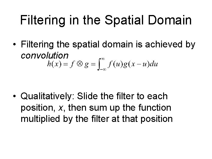
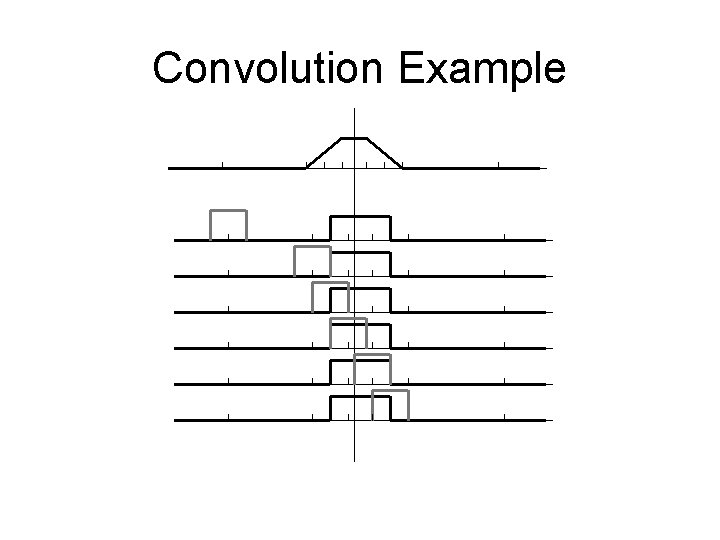
Filtering in the Spatial Domain • Filtering the spatial domain is achieved by convolution • Qualitatively: Slide the filter to each position, x, then sum up the function multiplied by the filter at that position

Convolution Example

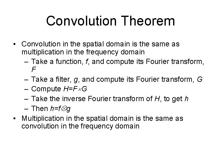
Convolution Theorem • Convolution in the spatial domain is the same as multiplication in the frequency domain – Take a function, f, and compute its Fourier transform, F – Take a filter, g, and compute its Fourier transform, G – Compute H=F G – Take the inverse Fourier transform of H, to get h – Then h=f g • Multiplication in the spatial domain is the same as convolution in the frequency domain

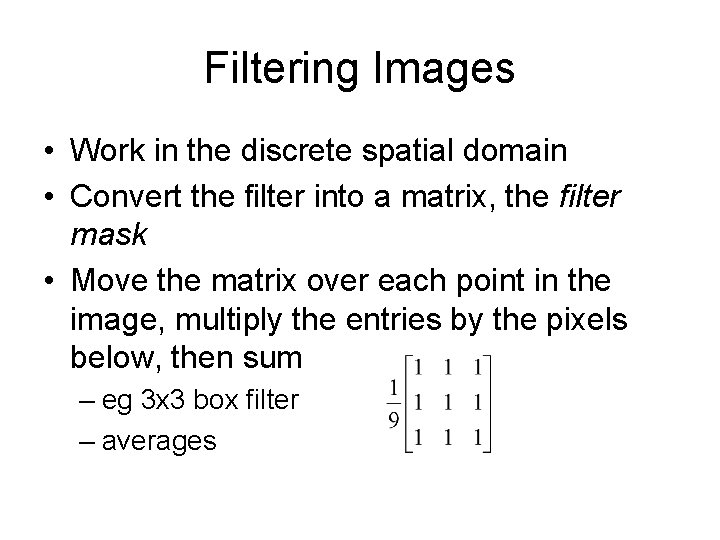
Filtering Images • Work in the discrete spatial domain • Convert the filter into a matrix, the filter mask • Move the matrix over each point in the image, multiply the entries by the pixels below, then sum – eg 3 x 3 box filter – averages

• filter 2(filter, image, shape) • filter 2(filter, image, 'same') is the default; it produces a matrix of equal size to the original image matrix. • filter 2(filter, image, 'valid') applies the mask only to inside pixels. • filter 2(filter, image, 'full') returns a result larger than the original; it does this by padding with zero, and applying the lter at all places on and around the image where the mask intersects the image matrix.

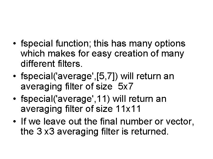
• fspecial function; this has many options which makes for easy creation of many different filters. • fspecial('average', [5, 7]) will return an averaging filter of size 5 x 7 • fspecial('average', 11) will return an averaging filter of size 11 x 11 • If we leave out the final number or vector, the 3 x 3 averaging filter is returned.

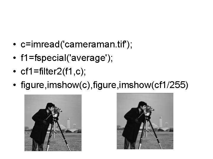
• • c=imread('cameraman. tif'); f 1=fspecial('average'); cf 1=filter 2(f 1, c); figure, imshow(c), figure, imshow(cf 1/255)

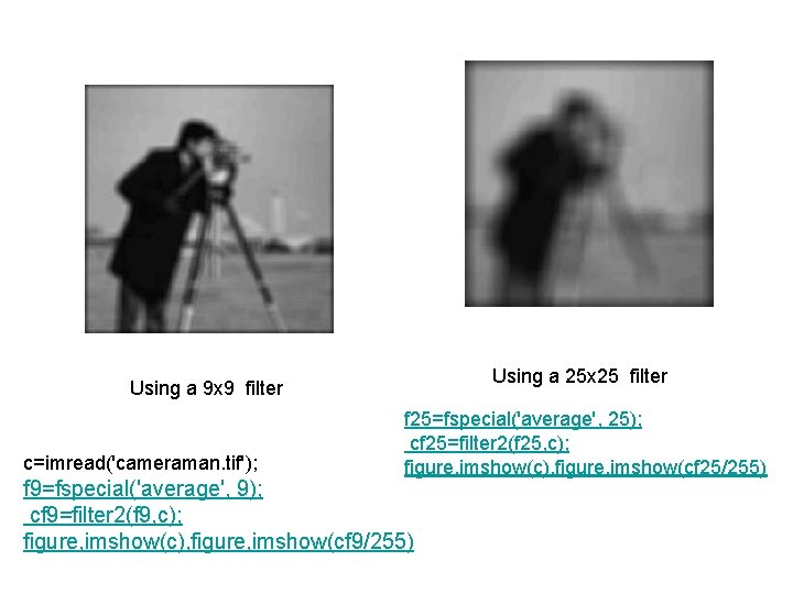
Using a 25 x 25 filter Using a 9 x 9 filter c=imread('cameraman. tif'); f 25=fspecial('average', 25); cf 25=filter 2(f 25, c); figure, imshow(c), figure, imshow(cf 25/255) f 9=fspecial('average', 9); cf 9=filter 2(f 9, c); figure, imshow(c), figure, imshow(cf 9/255)

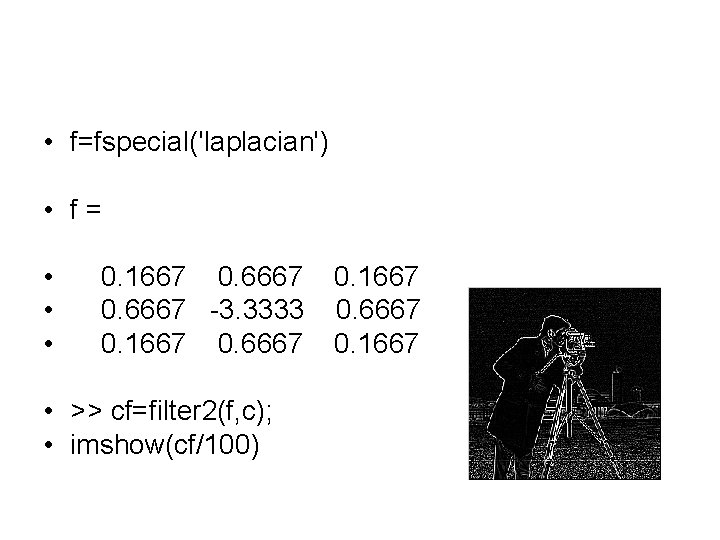
• f=fspecial('laplacian') • f= • • • 0. 1667 0. 6667 -3. 3333 0. 1667 0. 6667 • >> cf=filter 2(f, c); • imshow(cf/100) 0. 1667 0. 6667 0. 1667

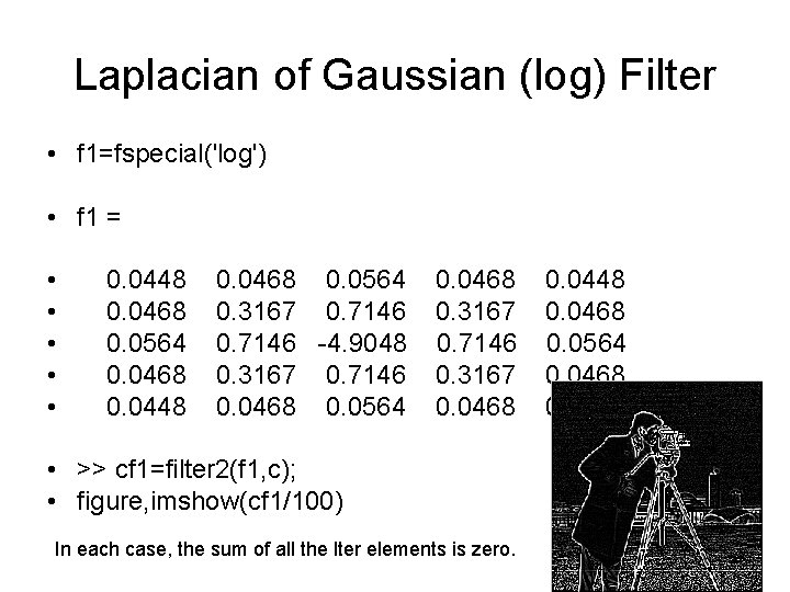
Laplacian of Gaussian (log) Filter • f 1=fspecial('log') • f 1 = • • • 0. 0448 0. 0468 0. 0564 0. 0468 0. 0448 0. 0468 0. 0564 0. 3167 0. 7146 -4. 9048 0. 3167 0. 7146 0. 0468 0. 0564 0. 0468 0. 3167 0. 7146 0. 3167 0. 0468 • >> cf 1=filter 2(f 1, c); • figure, imshow(cf 1/100) In each case, the sum of all the lter elements is zero. 0. 0448 0. 0468 0. 0564 0. 0468 0. 0448

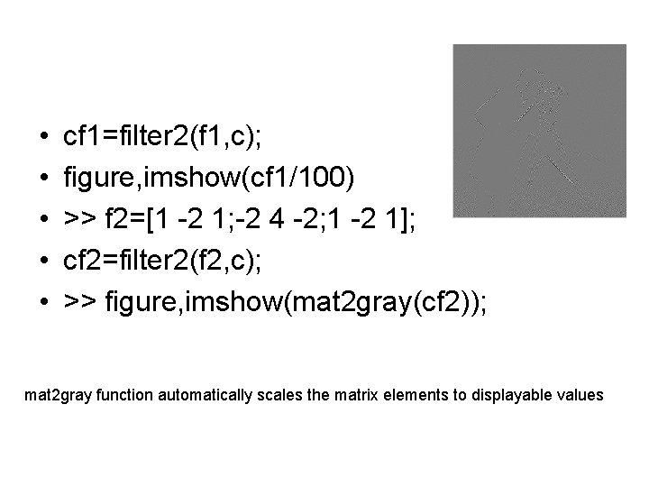
• • • cf 1=filter 2(f 1, c); figure, imshow(cf 1/100) >> f 2=[1 -2 1; -2 4 -2; 1 -2 1]; cf 2=filter 2(f 2, c); >> figure, imshow(mat 2 gray(cf 2)); mat 2 gray function automatically scales the matrix elements to displayable values

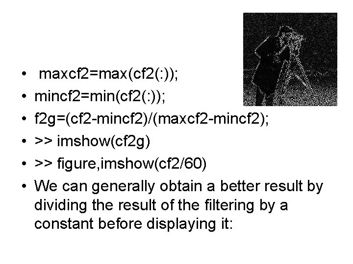
• • • maxcf 2=max(cf 2(: )); mincf 2=min(cf 2(: )); f 2 g=(cf 2 -mincf 2)/(maxcf 2 -mincf 2); >> imshow(cf 2 g) >> figure, imshow(cf 2/60) We can generally obtain a better result by dividing the result of the filtering by a constant before displaying it:

• a=50; s=3; • g=fspecial('gaussian', [a a], s); • surf(1: a, g)

• s=9; • >> g 2=fspecial('gaussian', [a a], s); • >> figure, surf(1: a, g 2)

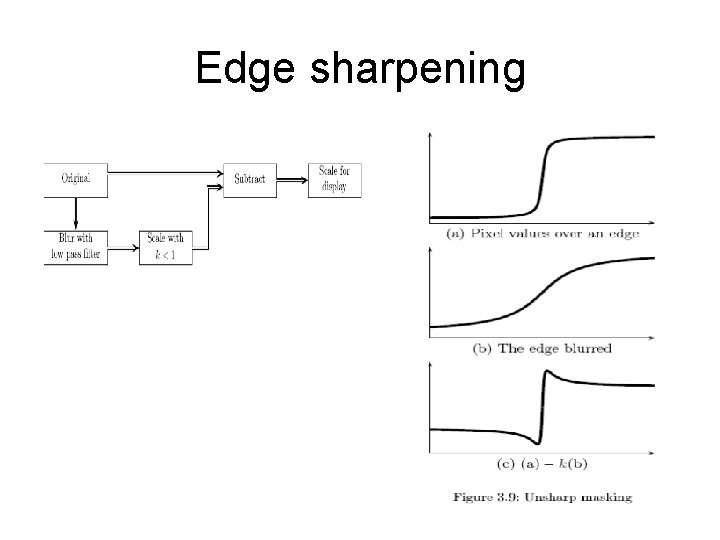
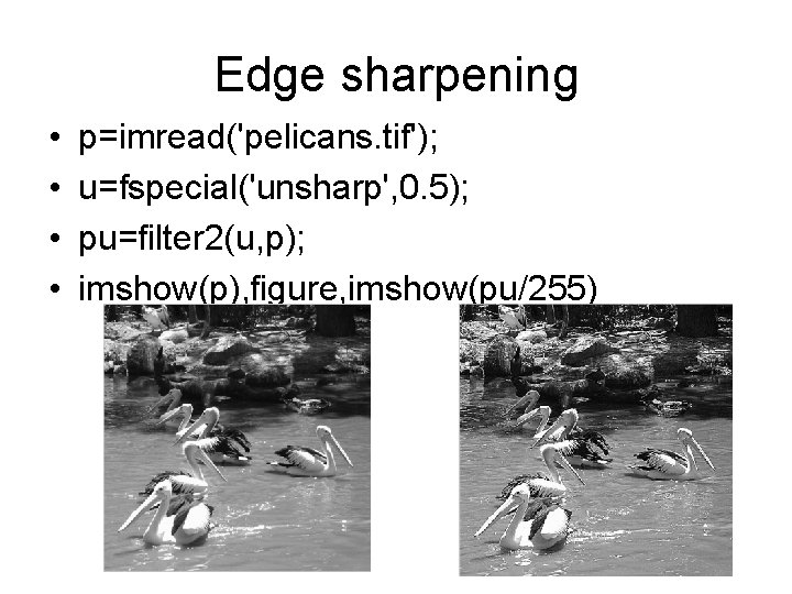
Edge sharpening

Edge sharpening • • p=imread('pelicans. tif'); u=fspecial('unsharp', 0. 5); pu=filter 2(u, p); imshow(p), figure, imshow(pu/255)

Non-linear Filters • maximum filter, which has as its output the maximum value • minimum filter, which has as its output the minimum value • rank-order filters. In such a filter, the elements under the mask are ordered • Colfilt function, which rearranges the image into columns first. • median filter, which takes the central value of the ordered list.

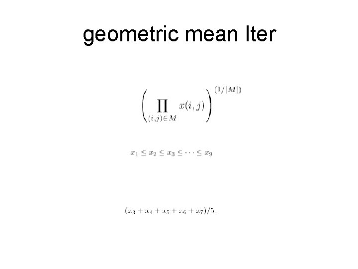
geometric mean lter