Filtering I Dr Chang Shu COMP 4900 C

Filtering (I) Dr. Chang Shu COMP 4900 C Winter 2008

Agenda • Getting to know images. • Image noise. • Image filters.

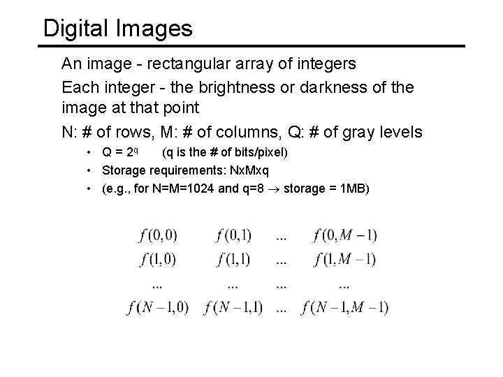
Digital Images An image - rectangular array of integers Each integer - the brightness or darkness of the image at that point N: # of rows, M: # of columns, Q: # of gray levels • Q = 2 q (q is the # of bits/pixel) • Storage requirements: Nx. Mxq • (e. g. , for N=M=1024 and q=8 storage = 1 MB)

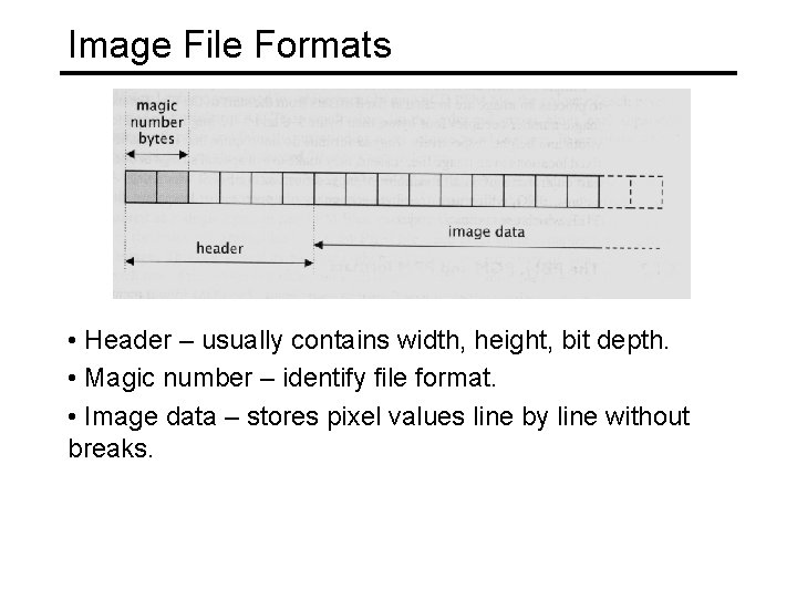
Image File Formats • Header – usually contains width, height, bit depth. • Magic number – identify file format. • Image data – stores pixel values line by line without breaks.

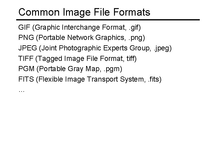
Common Image File Formats GIF (Graphic Interchange Format, . gif) PNG (Portable Network Graphics, . png) JPEG (Joint Photographic Experts Group, . jpeg) TIFF (Tagged Image File Format, tiff) PGM (Portable Gray Map, . pgm) FITS (Flexible Image Transport System, . fits) …

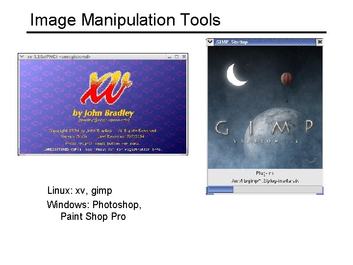
Image Manipulation Tools Linux: xv, gimp Windows: Photoshop, Paint Shop Pro

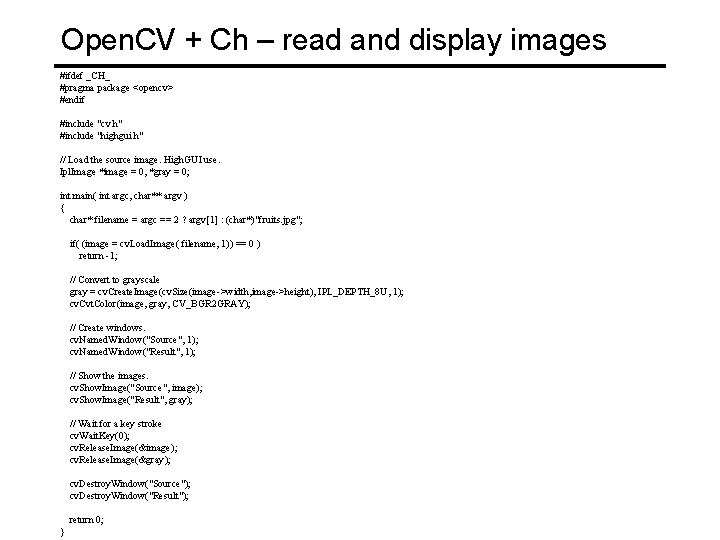
Open. CV + Ch – read and display images #ifdef _CH_ #pragma package <opencv> #endif #include "cv. h" #include "highgui. h" // Load the source image. High. GUI use. Ipl. Image *image = 0, *gray = 0; int main( int argc, char** argv ) { char* filename = argc == 2 ? argv[1] : (char*)"fruits. jpg"; if( (image = cv. Load. Image( filename, 1)) == 0 ) return -1; // Convert to grayscale gray = cv. Create. Image(cv. Size(image->width, image->height), IPL_DEPTH_8 U, 1); cv. Cvt. Color(image, gray, CV_BGR 2 GRAY); // Create windows. cv. Named. Window("Source", 1); cv. Named. Window("Result", 1); // Show the images. cv. Show. Image("Source", image); cv. Show. Image("Result", gray); // Wait for a key stroke cv. Wait. Key(0); cv. Release. Image(&image); cv. Release. Image(&gray); cv. Destroy. Window("Source"); cv. Destroy. Window("Result"); return 0; }

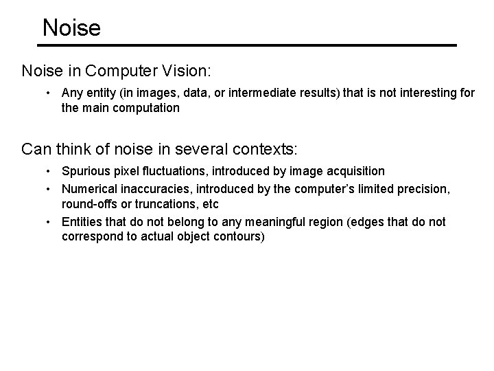
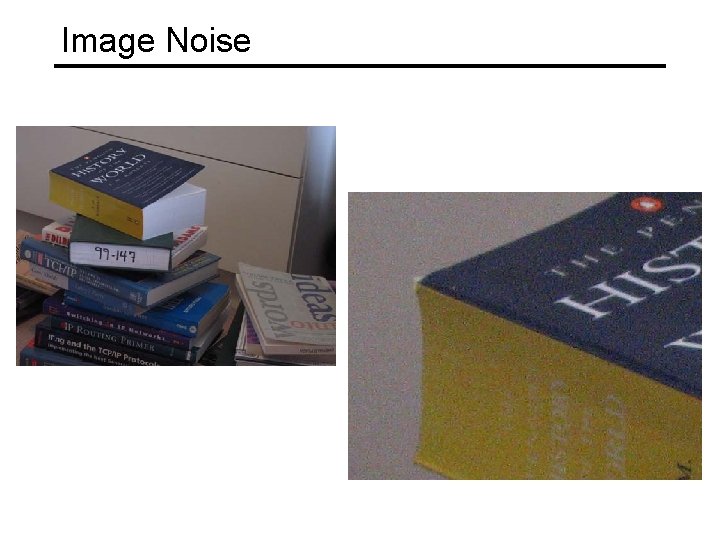
Noise in Computer Vision: • Any entity (in images, data, or intermediate results) that is not interesting for the main computation Can think of noise in several contexts: • Spurious pixel fluctuations, introduced by image acquisition • Numerical inaccuracies, introduced by the computer’s limited precision, round-offs or truncations, etc • Entities that do not belong to any meaningful region (edges that do not correspond to actual object contours)

Image Noise

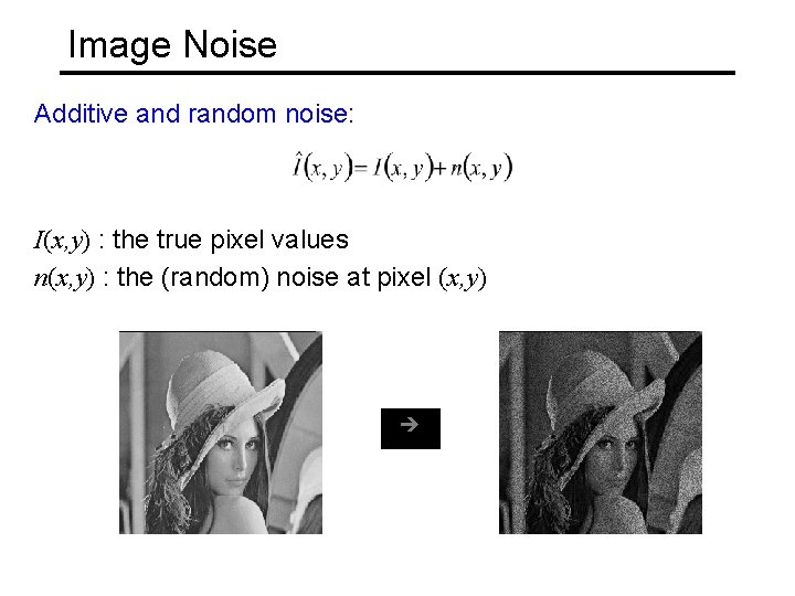
Image Noise Additive and random noise: I(x, y) : the true pixel values n(x, y) : the (random) noise at pixel (x, y)

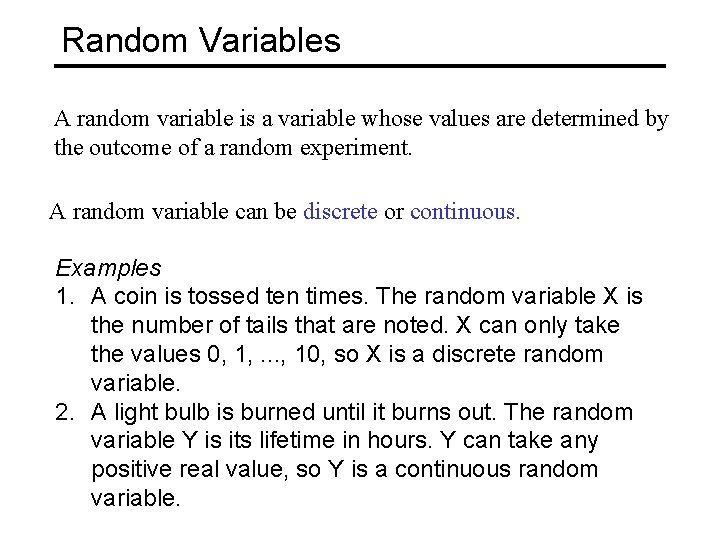
Random Variables A random variable is a variable whose values are determined by the outcome of a random experiment. A random variable can be discrete or continuous. Examples 1. A coin is tossed ten times. The random variable X is the number of tails that are noted. X can only take the values 0, 1, . . . , 10, so X is a discrete random variable. 2. A light bulb is burned until it burns out. The random variable Y is its lifetime in hours. Y can take any positive real value, so Y is a continuous random variable.

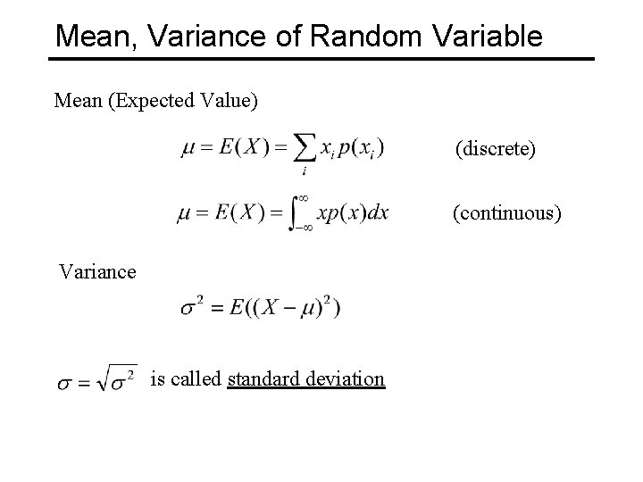
Mean, Variance of Random Variable Mean (Expected Value) (discrete) (continuous) Variance is called standard deviation

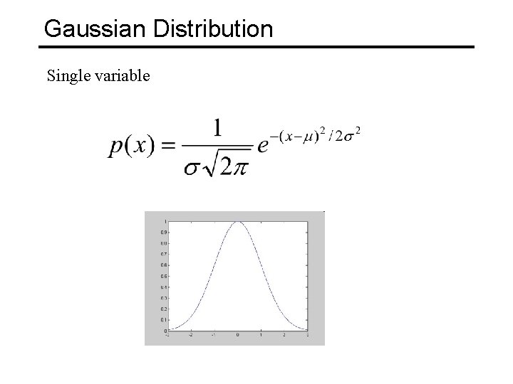
Gaussian Distribution Single variable

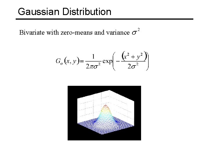
Gaussian Distribution Bivariate with zero-means and variance

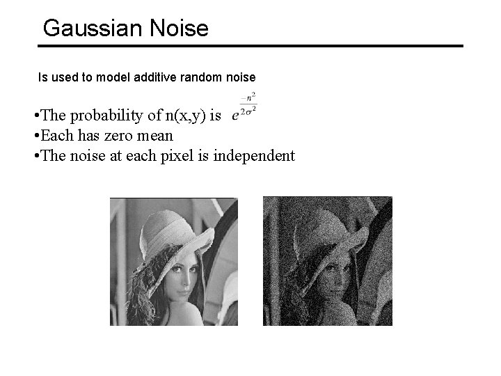
Gaussian Noise Is used to model additive random noise • The probability of n(x, y) is • Each has zero mean • The noise at each pixel is independent

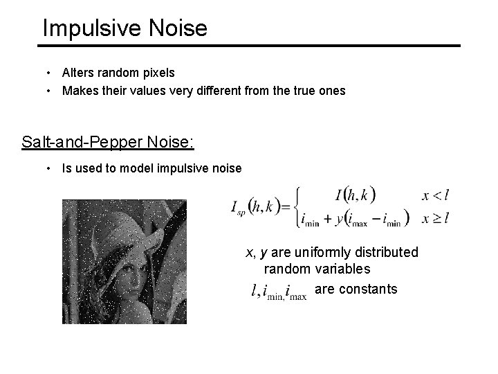
Impulsive Noise • Alters random pixels • Makes their values very different from the true ones Salt-and-Pepper Noise: • Is used to model impulsive noise x, y are uniformly distributed random variables are constants