Filaments in the Galaxy Their properties and their

Filaments in the Galaxy: Their properties and their connection with Star Formation Eugenio Schisano – IFSI INAF - Roma In collaboration with D. Polychroni, S. Molinari, D. Elia, M. Pestalozzi, G. Busquet, K. Rygl, N. Billot, M. Veneziani, and other members of Hi-GAL Team Background: Hi-GAL map of l=299° observed at 250 μm

Outline MIPS 24 μm

MIPS 24 μm

SPIRE 250 μm

MIPS 24 μm

SPIRE 250 μm

Pre-Herschel Observations in optical, near-IR, submm and in CO rotational lines show that gas and dust in the star forming complexes are arranged in a filamentary pattern. Either dense cores or more evolved objects, e. g. protostars, are found along such structures. Lynds 1962, Scheider & Elmegreen 1979, Mitchell et al. 2001, Loren 1989, Motte et al. 1998, Hartmann et al. 2002, Hatchell et al. 2005, Lada et al. 2007, Goldsmith et al. 2008, and many other works L 1495 For Example: Taurus Complex in 13 CO J = 1 - 0 L 1521 3 parallel filaments plus other coming out from the “hub” L 1495 L 1508 Figure from Goldsmith et al. 2008 (colors traces integrated intensities in 3 -5 km s-1 blue, 5 -7 km s-1 green 7 -9 km s-1 red) L 1536 5 pc

Herschel reminded us that the Molecular Clouds are strongly filamentary (Andrè et al. 2010, Molinari et al. 2010). Even if it is not a new idea, the scientific comunity is finally accepting that the spheroidal models are not adequate to describe star forming molecular clouds on large scales. Most of the recent numerical simulations are able to predict qualitatively the formation of a filament or a network of filaments in the process of forming stars (Nagai et al. 1998, Klessen 2001, Padoan et al. 2001, Klessen et al. 2004, Bernarjee et al. 2006, Li & Nakamura 2006, Vazques-Semadeni et al. 2007, Heitsch et al. 2008). So far Quantitative studies regard the cores (i. e. Offner & Krumoltz 2009)

Filaments are ubiquitous and represent an initial stage of star formation that is not well studied nor understood. Why do Molecular Clouds have those shapes? -) Result of the collision of randomly directed flows like large scale turbulence (Padoan et al. 2001, Klessen et al. 2004). -) Collision of uniform cylinders of gas along their symmetry axis (Vasquez-Semademi et al. 2007, Heitsch et al. 2008) -) Magnetically dominated model, where the self-gravity pulls gas to the midplane and ambipolar diffusion allows gravitational instabilities (Nakamura & Li 2008) Moreover, has the filamentary pattern any connection with the final cores/clumps ?

L 59 field SPIRE 250 μm map Highly structured Emission Difficulties in the extraction of compact objects 120’

L 59 field SPIRE 250 μm map Highly structured Emission Difficulties in the extraction of compact objects rk o tw s e x n ture e l p truc m Co subs of Image credit: Molinari 2010 Candidate source With the aid of an high pass band filter the emission Is damped. Dense compact structures start to stick out! Qualitatively the sources cluster on the filaments.

Our goal is to use the potential of Hi-GAL survey to build up a catalog of filamentary structures identified on the GP maps, for which we determine: Morphological Properties (position, length and width) linked to the filament formation process (sweeping/compression of matter, fragmentation etc). Physical Properties (mass, virial mass per unit length, temperature, column density) Mechanisms active in such structures. Study the stability of those structures. Comparison with classical filament models (Ostriker et al. 1964, Fiege & Pudritz 2000, 2004) of bounded, self-gravitating, structure. Correlation with the embedded cores (core shapes, core elongation, cores reciprocal distances – scales of filament fragmentation)

Identify a sample of filaments in unbiased way Measure Morphological and Physical properties Search for correlations with compact object properties

Filament identification Algorithm Image processing techniques to develop algorithms able to identify the filamentary structures. It is a classical “Pattern recognition problem”. Different approaches can be found in literature: 1) Optimal filtering: Attempt to find linear image structures from optimal edge detection, like Canny detector (see also Canny 1986). 2) Determination of the local properties of the image - Hessian Based methods: Compute the Hessian matrix and its eigenvalues to classify pixels on the basis of how cylinder like are the local intensities. - Topological analysis, like Dis. Per. SE code (see Sousbie 2010, Arzoumanian’s talk) 3) Other methods based on statistical estimators

Filament identification Algorithm Image processing techniques to develop algorithms able to identify the filamentary structures. It is a classical “Pattern recognition problem”. Different approaches can be found in literature: 1) Optimal filtering: Attempt to find linear image structures from optimal edge detection, like Canny detector (see also Canny 1986). 2) Determination of the local properties of the image - Hessian Based methods: Compute the Hessian matrix and its eigenvalues to classify pixels on the basis of how cylinder like are the local intensities. - Topological analysis, like Dis. Per. SE code (see Sousbie 2010, Arzoumanian’s talk) 3) Other methods based on statistical estimators

Filament identification Algorithm Image processing techniques to develop algorithms able to identify the filamentary structures. It is a classical “Pattern recognition problem”. Different approaches can be found in literature: 1) Optimal filtering: Attempt to find linear image structures from optimal edge detection, like Canny detector (see also Canny 1986). 2) Determination of the local properties of the image - Hessian Based methods: Compute the Hessian matrix and its eigenvalues to classify pixels on the basis of how cylinder like are the local intensities. - Topological analysis, like Dis. Per. SE code (see Sousbie 2010, Arzoumanian’s talk) 3) Other methods based on statistical estimators

Filament identification in a nutshell - 1 Filament: Structure that is concave down along two different principal axes and is almost flat in the other one. Method used on cosmological datasets to identify underlying structures (Aragon-Calvo et al. 2007, Bond et al 2010) Elongated cylindrical-like patterns are traced by the lowest eigenvalue (λ 1 << λ 2) and the eigenvectors (A 1, A 2) of the Hessian matrix computed in each pixel. Extended not elongated regions are rejected by criteria on the highest eigenvalue and the eigenvectors. However the method may miss structures with large variations of emission along the axis of the cylinder ( flat condition along filament axis often are not fulfilled )

Filament identification in a nutshell - 2 We complements the Hessian approach with an Edge Dectector-type method. We compute the eigenvalues of the Hessian Matrix and determine a threshold value to identify the pixels belonging to the filament. Assuming that the Filament is symmetric in its shape we apply the morphological operators of erosion (Gonzales & Wood 2002) to determine an estimate of the central “Spine” (see also Qu & Shih 2005) All the points of the “Spine” are then connected through a Minimum Spanning Tree (MST) that give the unique path linking together all the pixels of the spine.

Input Image Eigenvalues of the Hessian Matrix Filament identification in a nutshell - 2 We compute the eigenvalues of the Hessian Matrix and determine a threshold value to identify the pixels belonging to the filament. Assuming that the Filament is symmetric in its shape we apply the morphological operators of erosion (Gonzales & Wood 2002) to determine an estimate of the central “Spine” (see also Qu & Shih 2005) Simulation Filament with 2 sources Contrast Filament – Background ~ 9 Thresholded mask Application Morphological Operator

Filament Simulations We build up a simple simulation of of linear structures. The filaments are simulated by computing spines with moderate curvatures, idealized radial profile with a power-law decrement with exponent between 2 and 4. Variable intensity along the spine Introduced to take in account the presence of sources embedded in the structure. Structures of different widths and lengths are distributed on a FBM map (Stutzki et al. 1998) simulating the emission of the diffuse ISM Fluctuation on the Spine

Filament Simulations Black lines define the spine of the linear structures identified by mixing Hessian Diagonalization methods with “edge detectors” approaches. Areas are recovered within 15% the simulated region, projected lengths with accuracy of 5 to 10%. Fluctuation on the Spine

Identify a sample of filaments in unbiased way Measure Morphological and Physical properties Search for correlations with compact object properties

A case of study - L 59 region MIPS 24 μm Vulpecula region Well know filamentary regions. Vulpecula OB 1 association. NGC 6823 10’ See Billot et al. 2010, Elia et al. 2010

A case of study - L 59 region PACS 160 μm 10’ SPIRE 250μm μm 10’ Using the photometry package Cu. TEx (Molinari et al. 2010) we identified the compact sources in the Vulpecula field. Improvement in the extraction techniques allowed us to find 401 candidates with robust indipendent detection in the 3 consecutive bands of 160, 250, 350 μm.

A case of study - L 59 region SPIRE 250 μm 10’ Source detected By Cu. TEx in at least 3 phtoometryc band

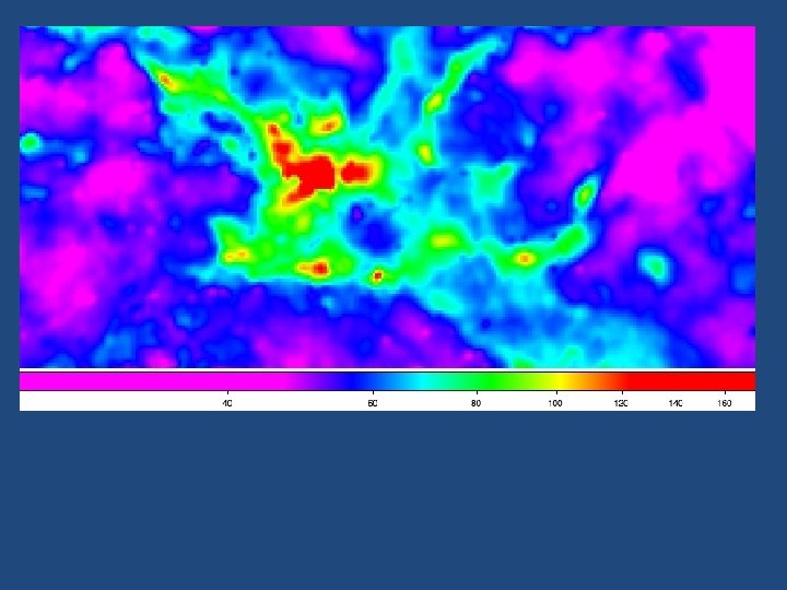
A case of study - L 59 region AV (mag) SPIRE 250 μm 10’ We computed the Column Density and Temperature maps fitting modified gray body functions by pixel. Quite a few filaments are recognized on the column density map.

A case of study - L 59 region Temperature Map

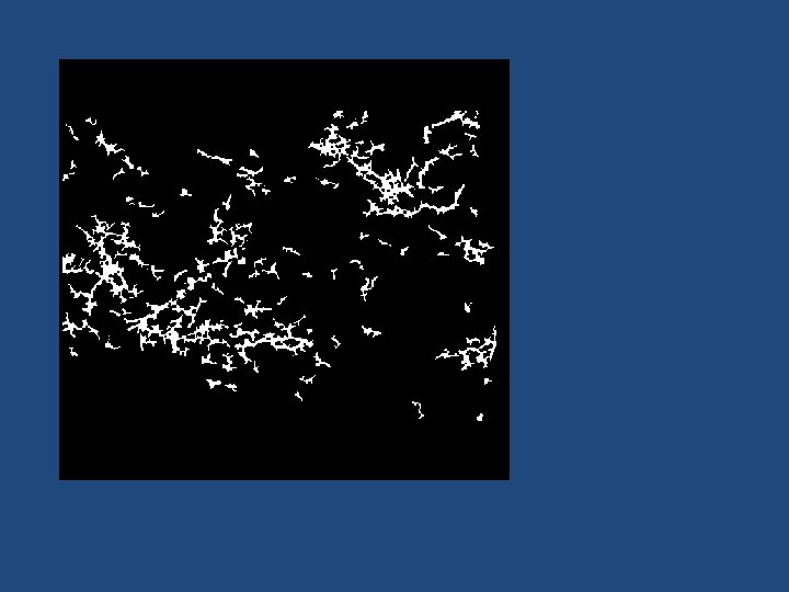
A case of study - L 59 region AV (mag) We identied 50 filaments that have a mean length longer than 200”. ( > 2 pc @ 2. 2 kpc) Another 50 filaments are classified as candidates coherent structures since they are enough extended to be identified, but have shorter lengths than 200”. Original masks includes hundreds of small scale structures, highlighted by the derivative computatio. n 10’

Identify a sample of filaments in unbiased way Measure Morphological and Physical properties Search for correlations with compact object properties Low extinction regions with mean values of ~ 3 AV. Pixels associated with sources are not taken into account in those computation. Background is removed fitting neighbors pixels. Mean Temperature are roughtly constant. No systematic difference between long and short structures.

A case of study - L 59 region AV (mag) 10’

We fitted the radial profile of each filament computing the radial distance of each pixel from the identified spine. We mean the intensity of pixels with same radial distance in region 4 pixels wide. We find that quite a few filaments show a resolved radial profile with typical sizes of ~50” (0. 5 pc at 2. 2 kpc)

Identify a sample of filaments in unbiased way Measure Morphological and Physical properties Search for correlations with compact object properties

Yellow: Sources Detected Inside filament Red sources Outside filaments Adopting the catalog of the compact objects with detections at 3 bands 292 sources inside ~73 % 109 sources outside ~37 % However, considering the sources that are detected only at SPIRE wavelengths we find that the number of sources inside and outside filament are evenly splitted Still need to be investigated

Virial Parameter Map M / Mvir Virial parameter from 13 CO Galactic Ring Survey Data Bright regions are supercritical – correspond to the Cores/Clumps See also Andrè talk

Fraction of Dense matter distributed in filamentary region: All the observed higher density regions belong to filamentary regions ~50% of the matter with Av > 8 is identified as belonging to a source inside the filament Frea

Fraction of Dense matter distributed in filamentary region: If we include all the sources detected only at SPIRE wavelengths the fraction of dense matter found in sources inside the filaments Increase.

There indication that the number of sources increase with the filament Column Density Need to be confirmed from the analysis of more fields Denser Filament Fraction In Filaments Out Filaments With MIPS 24 μm 0. 53± 0. 08 Conterpart 0. 45± 0. 09 With PACS 70 μm 0. 43± 0. 07 Conterpart 0. 31± 0. 07 Sources with Excess at 70 μm 0. 56± 0. 20 0. 58± 0. 13

Conclusions Filaments are found everywhere in the Galaxy They have a strong connection with the process of Star Formation. We developed methods to identify the regions corresponding to the Filamentary structures and to extract physical parameters from them (sizes, lengths, masses) First analysis on one field of the Hi-GAL survey indicates that most of the dense matter is arranged in the filaments. Moreover, compact objects are found with more probability in those structures.