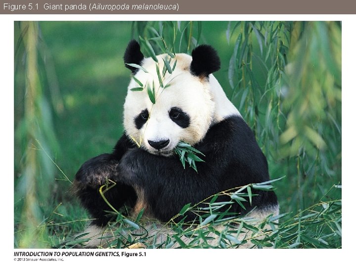
Figure 5 1 Giant panda Ailuropoda melanoleuca Figure

Figure 5. 1 Giant panda (Ailuropoda melanoleuca)

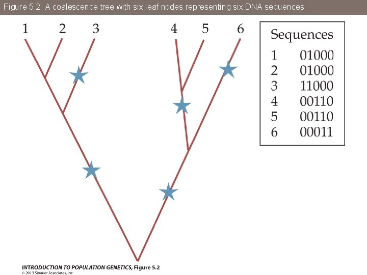
Figure 5. 2 A coalescence tree with six leaf nodes representing six DNA sequences

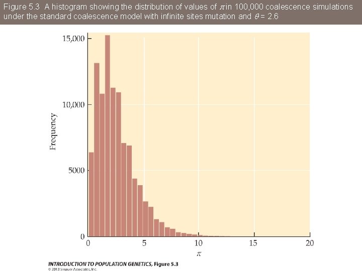
Figure 5. 3 A histogram showing the distribution of values of p in 100, 000 coalescence simulations under the standard coalescence model with infinite sites mutation and q = 2. 6

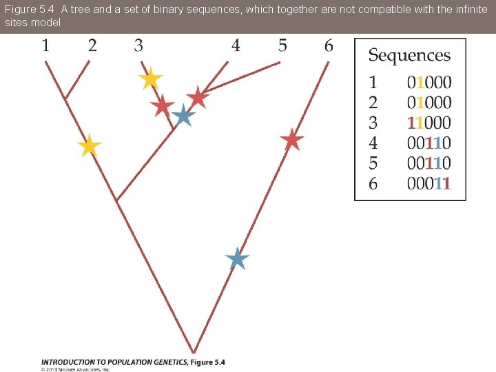
Figure 5. 4 A tree and a set of binary sequences, which together are not compatible with the infinite sites model

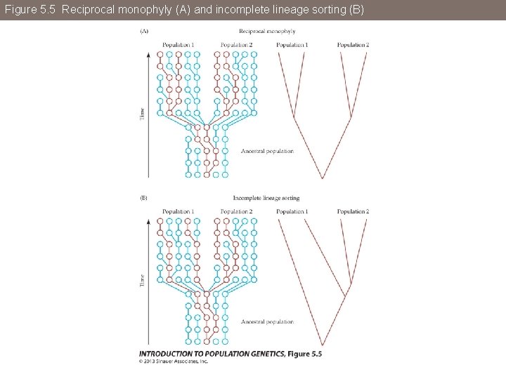
Figure 5. 5 Reciprocal monophyly (A) and incomplete lineage sorting (B)

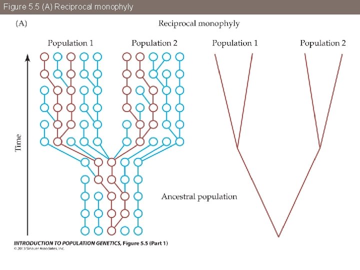
Figure 5. 5 (A) Reciprocal monophyly

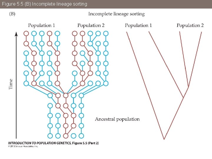
Figure 5. 5 (B) Incomplete lineage sorting

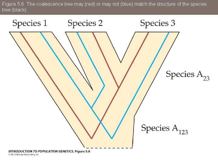
Figure 5. 6 The coalescence tree may (red) or may not (blue) match the structure of the species tree (black)

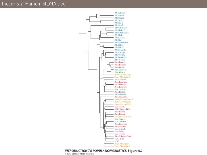
Figure 5. 7 Human mt. DNA tree

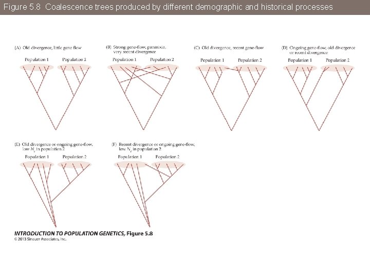
Figure 5. 8 Coalescence trees produced by different demographic and historical processes

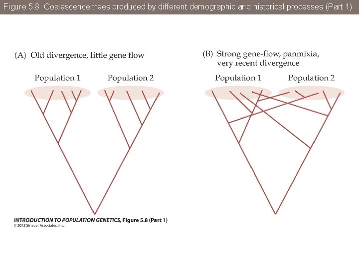
Figure 5. 8 Coalescence trees produced by different demographic and historical processes (Part 1)

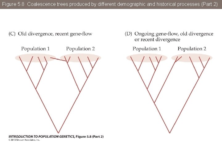
Figure 5. 8 Coalescence trees produced by different demographic and historical processes (Part 2)

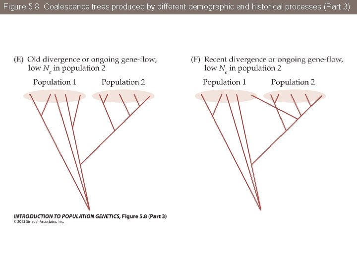
Figure 5. 8 Coalescence trees produced by different demographic and historical processes (Part 3)

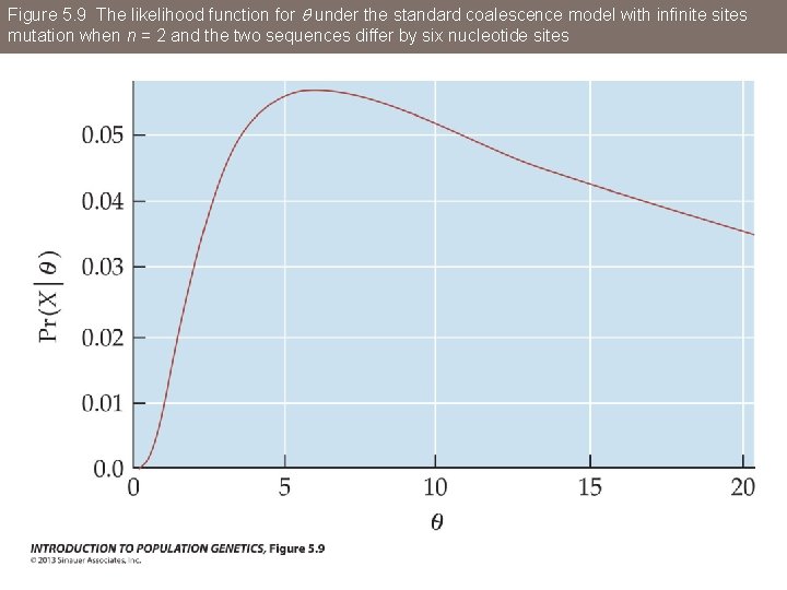
Figure 5. 9 The likelihood function for q under the standard coalescence model with infinite sites mutation when n = 2 and the two sequences differ by six nucleotide sites

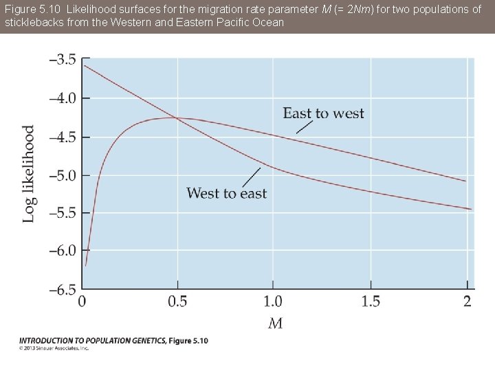
Figure 5. 10 Likelihood surfaces for the migration rate parameter M (= 2 Nm) for two populations of sticklebacks from the Western and Eastern Pacific Ocean

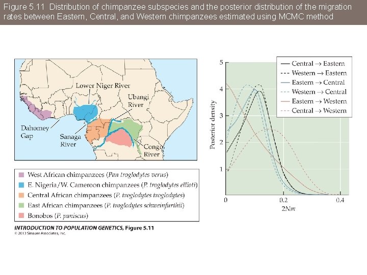
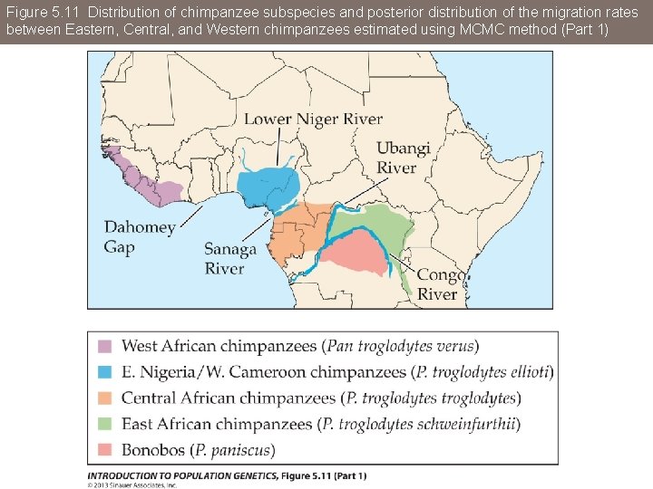
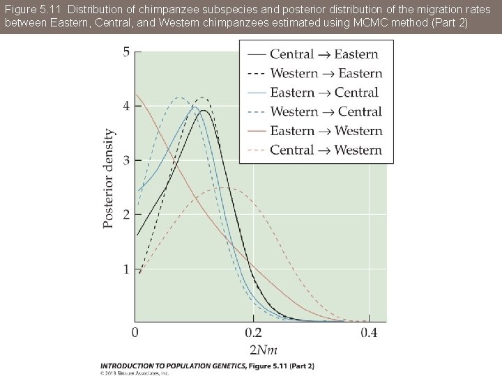
Figure 5. 11 Distribution of chimpanzee subspecies and the posterior distribution of the migration rates between Eastern, Central, and Western chimpanzees estimated using MCMC method

Figure 5. 11 Distribution of chimpanzee subspecies and posterior distribution of the migration rates between Eastern, Central, and Western chimpanzees estimated using MCMC method (Part 1)

Figure 5. 11 Distribution of chimpanzee subspecies and posterior distribution of the migration rates between Eastern, Central, and Western chimpanzees estimated using MCMC method (Part 2)

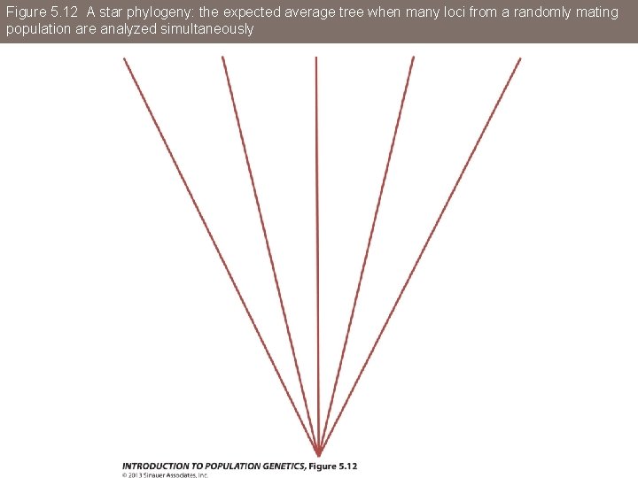
Figure 5. 12 A star phylogeny: the expected average tree when many loci from a randomly mating population are analyzed simultaneously

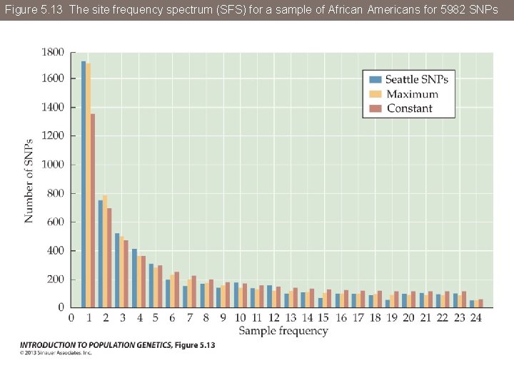
Figure 5. 13 The site frequency spectrum (SFS) for a sample of African Americans for 5982 SNPs

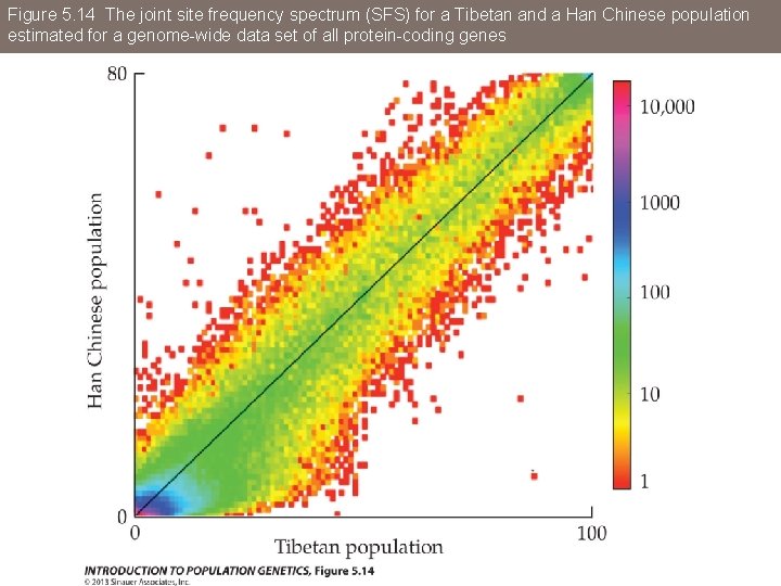
Figure 5. 14 The joint site frequency spectrum (SFS) for a Tibetan and a Han Chinese population estimated for a genome-wide data set of all protein-coding genes

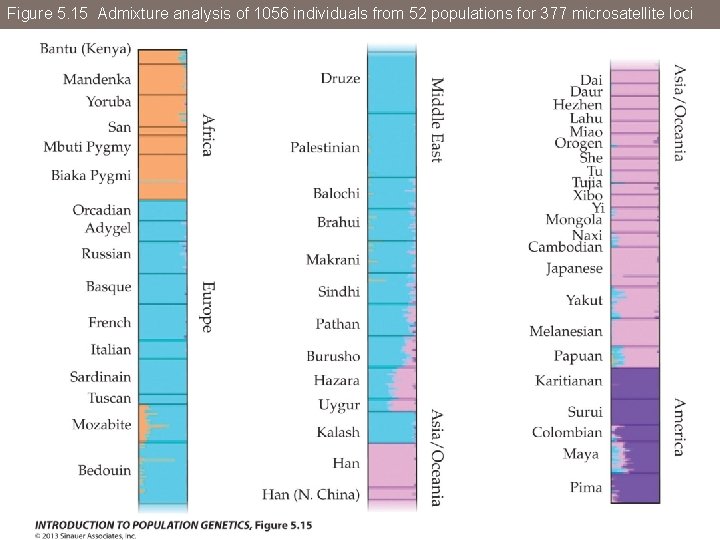
Figure 5. 15 Admixture analysis of 1056 individuals from 52 populations for 377 microsatellite loci

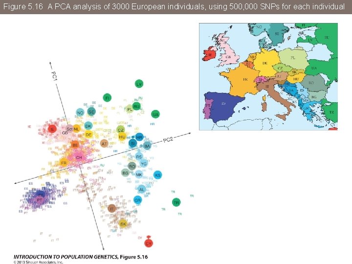
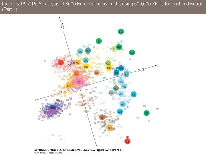
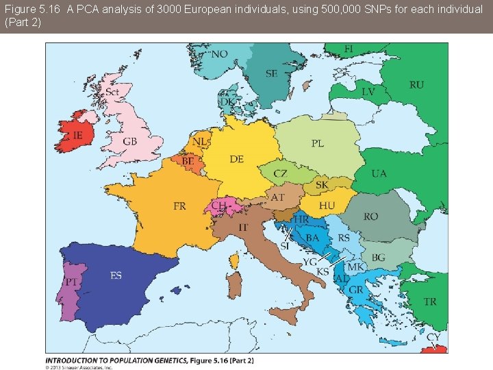
Figure 5. 16 A PCA analysis of 3000 European individuals, using 500, 000 SNPs for each individual

Figure 5. 16 A PCA analysis of 3000 European individuals, using 500, 000 SNPs for each individual (Part 1)

Figure 5. 16 A PCA analysis of 3000 European individuals, using 500, 000 SNPs for each individual (Part 2)

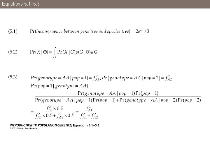
Equations 5. 1– 5. 3

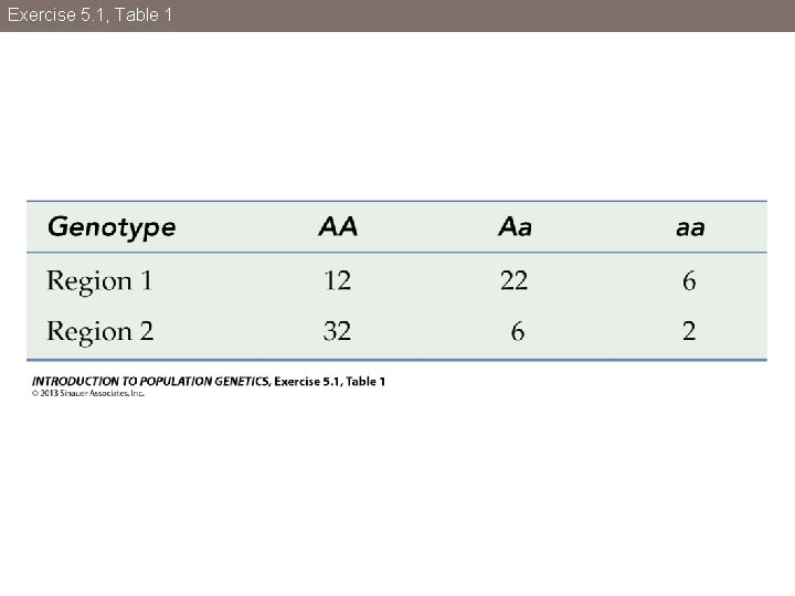
Exercise 5. 1, Table 1

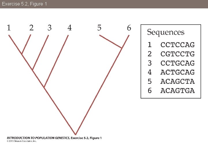
Exercise 5. 2, Figure 1