Figure 11 1 Linear system model for a
![Figure 11. 1 Linear system model for a signal s[n]. Discrete-Time Signal Processing, Third Figure 11. 1 Linear system model for a signal s[n]. Discrete-Time Signal Processing, Third](https://slidetodoc.com/presentation_image/9b9b1b9f6108e900cca5f9896739ae06/image-1.jpg)
![Figure 11. 4 Linear system model for a random signal s[n]. Discrete-Time Signal Processing, Figure 11. 4 Linear system model for a random signal s[n]. Discrete-Time Signal Processing,](https://slidetodoc.com/presentation_image/9b9b1b9f6108e900cca5f9896739ae06/image-4.jpg)
- Slides: 34
![Figure 11 1 Linear system model for a signal sn DiscreteTime Signal Processing Third Figure 11. 1 Linear system model for a signal s[n]. Discrete-Time Signal Processing, Third](https://slidetodoc.com/presentation_image/9b9b1b9f6108e900cca5f9896739ae06/image-1.jpg)
Figure 11. 1 Linear system model for a signal s[n]. Discrete-Time Signal Processing, Third Edition Alan V. Oppenheim • Ronald W. Schafer Copyright © 2010, © 1999, © 1989 by Pearson Education, Inc. All rights reserved.

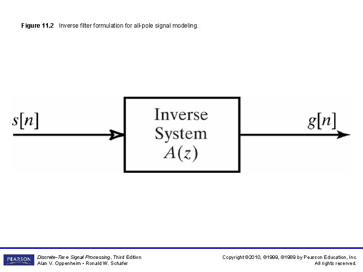
Figure 11. 2 Inverse filter formulation for all-pole signal modeling. Discrete-Time Signal Processing, Third Edition Alan V. Oppenheim • Ronald W. Schafer Copyright © 2010, © 1999, © 1989 by Pearson Education, Inc. All rights reserved.

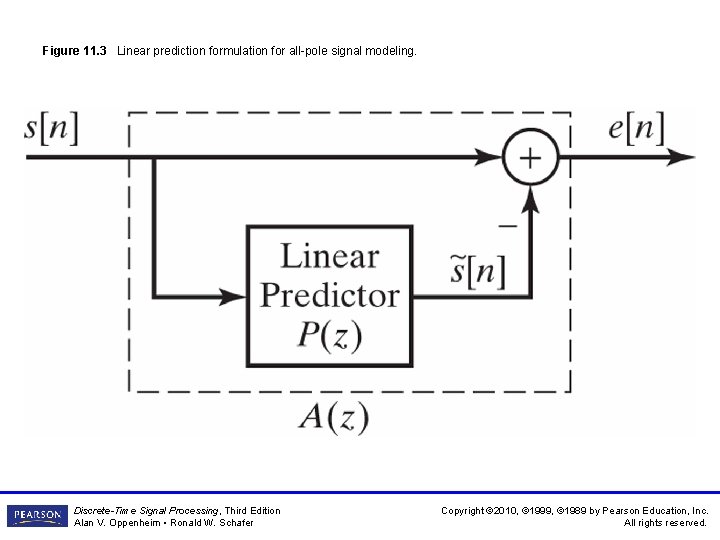
Figure 11. 3 Linear prediction formulation for all-pole signal modeling. Discrete-Time Signal Processing, Third Edition Alan V. Oppenheim • Ronald W. Schafer Copyright © 2010, © 1999, © 1989 by Pearson Education, Inc. All rights reserved.
![Figure 11 4 Linear system model for a random signal sn DiscreteTime Signal Processing Figure 11. 4 Linear system model for a random signal s[n]. Discrete-Time Signal Processing,](https://slidetodoc.com/presentation_image/9b9b1b9f6108e900cca5f9896739ae06/image-4.jpg)
Figure 11. 4 Linear system model for a random signal s[n]. Discrete-Time Signal Processing, Third Edition Alan V. Oppenheim • Ronald W. Schafer Copyright © 2010, © 1999, © 1989 by Pearson Education, Inc. All rights reserved.

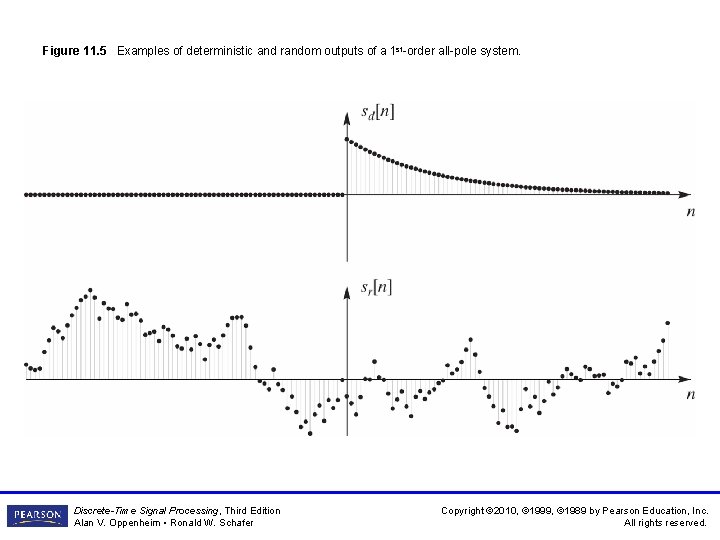
Figure 11. 5 Examples of deterministic and random outputs of a 1 st-order all-pole system. Discrete-Time Signal Processing, Third Edition Alan V. Oppenheim • Ronald W. Schafer Copyright © 2010, © 1999, © 1989 by Pearson Education, Inc. All rights reserved.

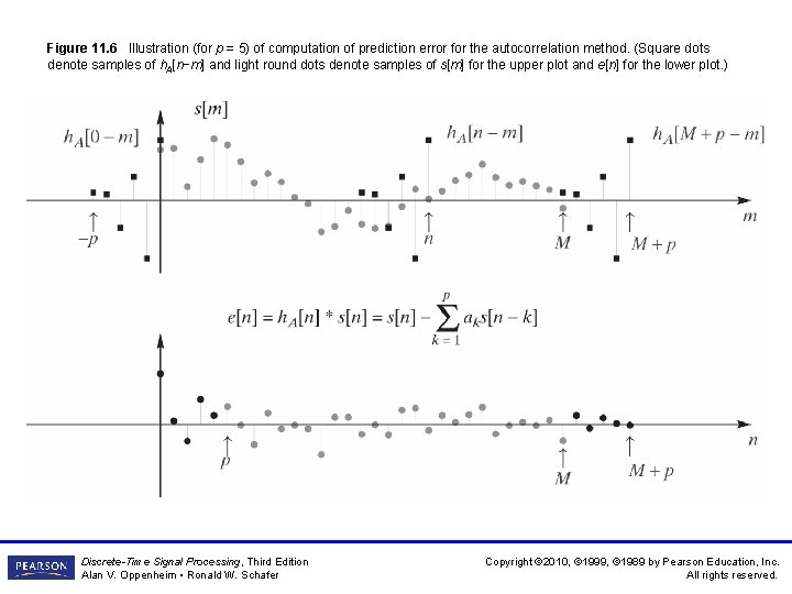
Figure 11. 6 Illustration (for p = 5) of computation of prediction error for the autocorrelation method. (Square dots denote samples of h. A[n−m] and light round dots denote samples of s[m] for the upper plot and e[n] for the lower plot. ) Discrete-Time Signal Processing, Third Edition Alan V. Oppenheim • Ronald W. Schafer Copyright © 2010, © 1999, © 1989 by Pearson Education, Inc. All rights reserved.

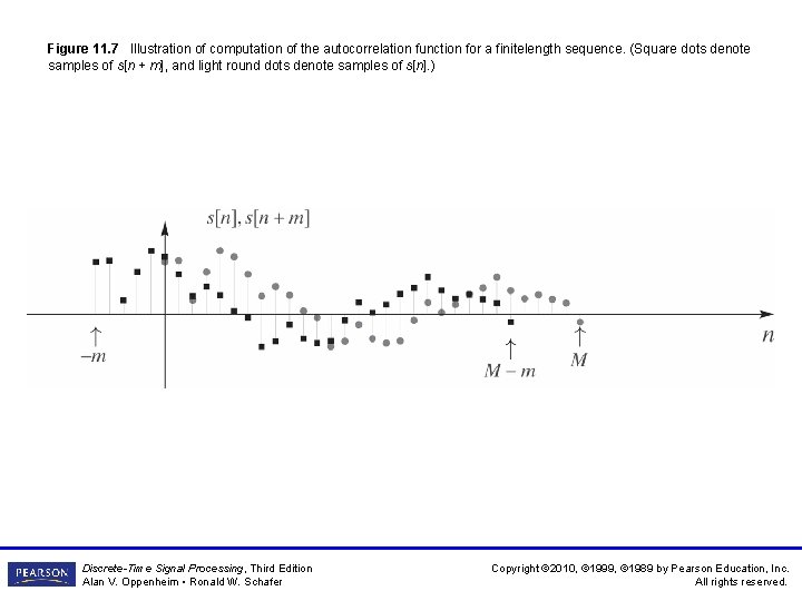
Figure 11. 7 Illustration of computation of the autocorrelation function for a finitelength sequence. (Square dots denote samples of s[n + m], and light round dots denote samples of s[n]. ) Discrete-Time Signal Processing, Third Edition Alan V. Oppenheim • Ronald W. Schafer Copyright © 2010, © 1999, © 1989 by Pearson Education, Inc. All rights reserved.

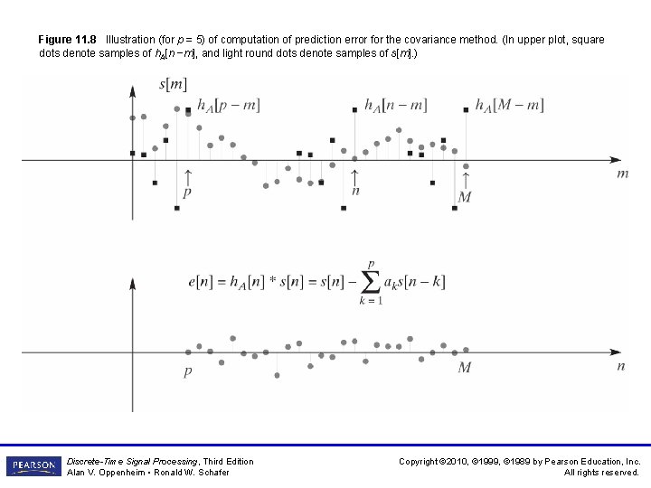
Figure 11. 8 Illustration (for p = 5) of computation of prediction error for the covariance method. (In upper plot, square dots denote samples of h. A[n −m], and light round dots denote samples of s[m]. ) Discrete-Time Signal Processing, Third Edition Alan V. Oppenheim • Ronald W. Schafer Copyright © 2010, © 1999, © 1989 by Pearson Education, Inc. All rights reserved.

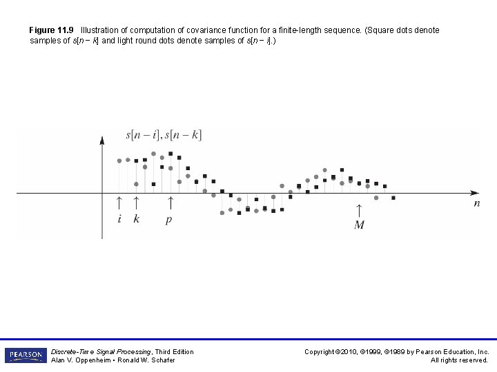
Figure 11. 9 Illustration of computation of covariance function for a finite-length sequence. (Square dots denote samples of s[n − k] and light round dots denote samples of s[n − i]. ) Discrete-Time Signal Processing, Third Edition Alan V. Oppenheim • Ronald W. Schafer Copyright © 2010, © 1999, © 1989 by Pearson Education, Inc. All rights reserved.

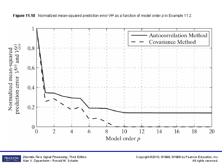
Figure 11. 10 Normalized mean-squared prediction error V(p) as a function of model order p in Example 11. 2. Discrete-Time Signal Processing, Third Edition Alan V. Oppenheim • Ronald W. Schafer Copyright © 2010, © 1999, © 1989 by Pearson Education, Inc. All rights reserved.

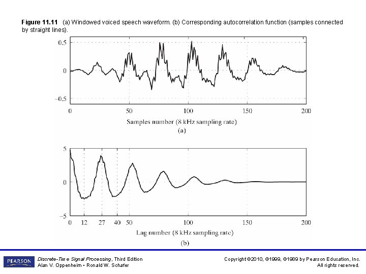
Figure 11. 11 (a) Windowed voiced speech waveform. (b) Corresponding autocorrelation function (samples connected by straight lines). Discrete-Time Signal Processing, Third Edition Alan V. Oppenheim • Ronald W. Schafer Copyright © 2010, © 1999, © 1989 by Pearson Education, Inc. All rights reserved.

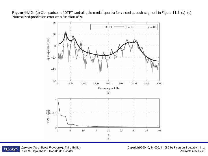
Figure 11. 12 (a) Comparison of DTFT and all-pole model spectra for voiced speech segment in Figure 11. 11(a). (b) Normalized prediction error as a function of p. Discrete-Time Signal Processing, Third Edition Alan V. Oppenheim • Ronald W. Schafer Copyright © 2010, © 1999, © 1989 by Pearson Education, Inc. All rights reserved.

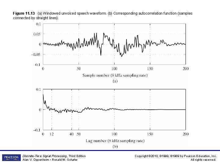
Figure 11. 13 (a) Windowed unvoiced speech waveform. (b) Corresponding autocorrelation function (samples connected by straight lines). Discrete-Time Signal Processing, Third Edition Alan V. Oppenheim • Ronald W. Schafer Copyright © 2010, © 1999, © 1989 by Pearson Education, Inc. All rights reserved.

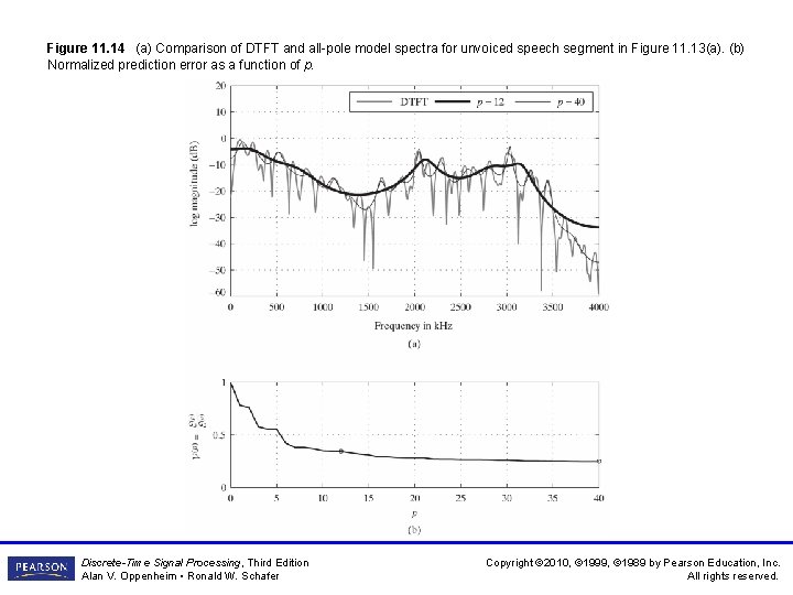
Figure 11. 14 (a) Comparison of DTFT and all-pole model spectra for unvoiced speech segment in Figure 11. 13(a). (b) Normalized prediction error as a function of p. Discrete-Time Signal Processing, Third Edition Alan V. Oppenheim • Ronald W. Schafer Copyright © 2010, © 1999, © 1989 by Pearson Education, Inc. All rights reserved.

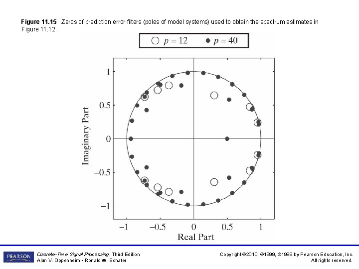
Figure 11. 15 Zeros of prediction error filters (poles of model systems) used to obtain the spectrum estimates in Figure 11. 12. Discrete-Time Signal Processing, Third Edition Alan V. Oppenheim • Ronald W. Schafer Copyright © 2010, © 1999, © 1989 by Pearson Education, Inc. All rights reserved.

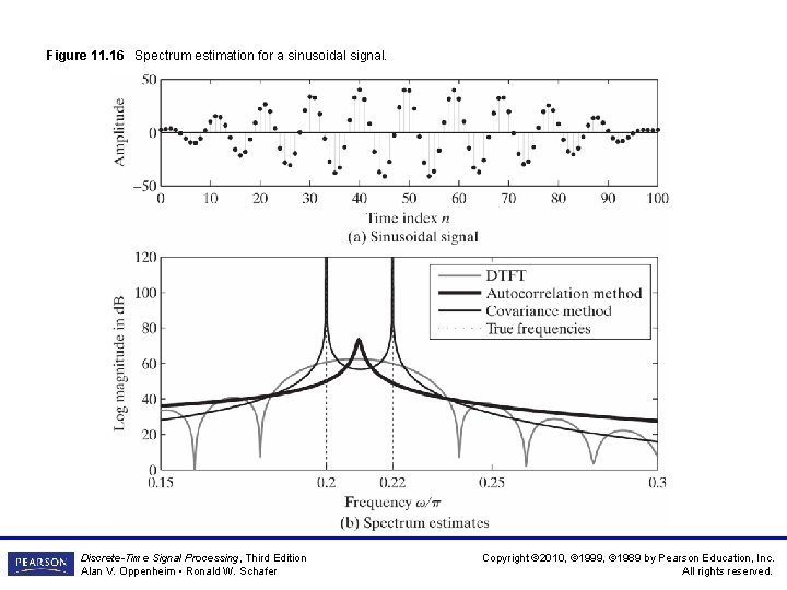
Figure 11. 16 Spectrum estimation for a sinusoidal signal. Discrete-Time Signal Processing, Third Edition Alan V. Oppenheim • Ronald W. Schafer Copyright © 2010, © 1999, © 1989 by Pearson Education, Inc. All rights reserved.

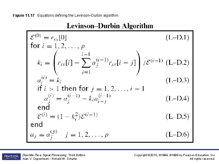
Figure 11. 17 Equations defining the Levinson–Durbin algorithm. Discrete-Time Signal Processing, Third Edition Alan V. Oppenheim • Ronald W. Schafer Copyright © 2010, © 1999, © 1989 by Pearson Education, Inc. All rights reserved.

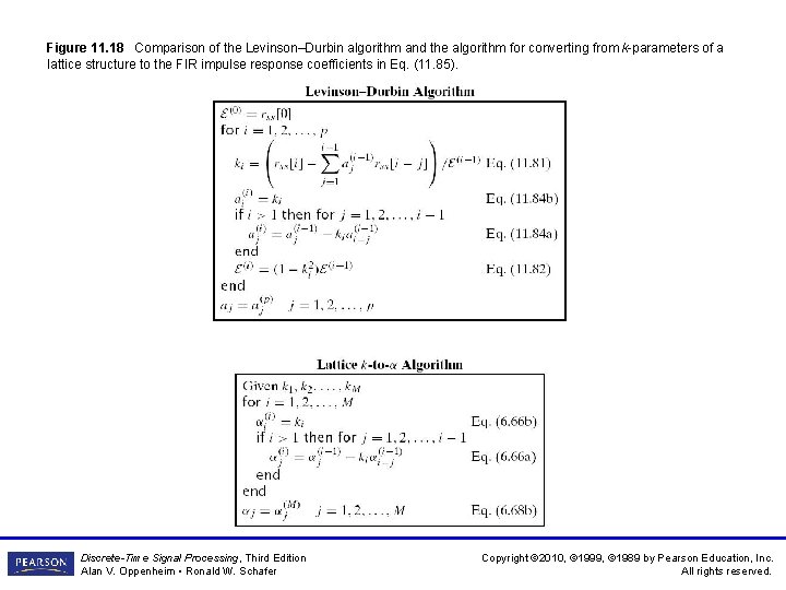
Figure 11. 18 Comparison of the Levinson–Durbin algorithm and the algorithm for converting from k-parameters of a lattice structure to the FIR impulse response coefficients in Eq. (11. 85). Discrete-Time Signal Processing, Third Edition Alan V. Oppenheim • Ronald W. Schafer Copyright © 2010, © 1999, © 1989 by Pearson Education, Inc. All rights reserved.

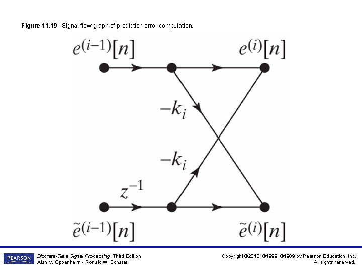
Figure 11. 19 Signal flow graph of prediction error computation. Discrete-Time Signal Processing, Third Edition Alan V. Oppenheim • Ronald W. Schafer Copyright © 2010, © 1999, © 1989 by Pearson Education, Inc. All rights reserved.

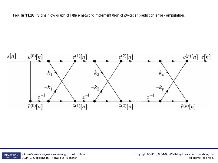
Figure 11. 20 Signal flow graph of lattice network implementation of pth-order prediction error computation. Discrete-Time Signal Processing, Third Edition Alan V. Oppenheim • Ronald W. Schafer Copyright © 2010, © 1999, © 1989 by Pearson Education, Inc. All rights reserved.

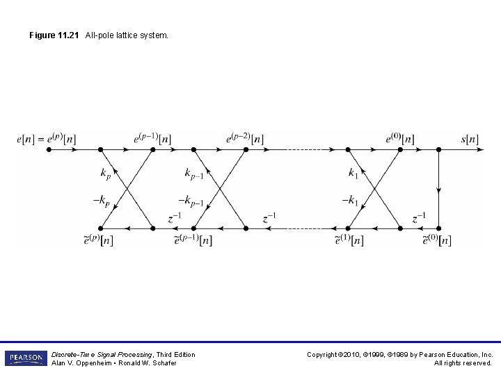
Figure 11. 21 All-pole lattice system. Discrete-Time Signal Processing, Third Edition Alan V. Oppenheim • Ronald W. Schafer Copyright © 2010, © 1999, © 1989 by Pearson Education, Inc. All rights reserved.

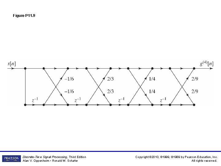
Figure P 11. 9 Discrete-Time Signal Processing, Third Edition Alan V. Oppenheim • Ronald W. Schafer Copyright © 2010, © 1999, © 1989 by Pearson Education, Inc. All rights reserved.

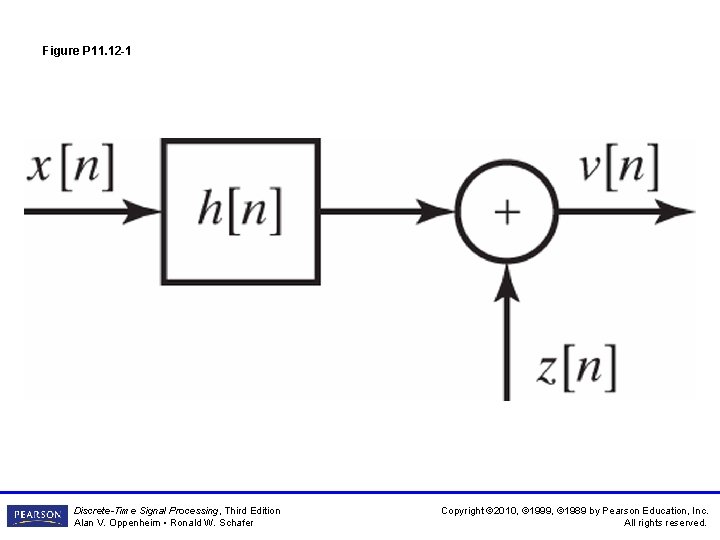
Figure P 11. 12 -1 Discrete-Time Signal Processing, Third Edition Alan V. Oppenheim • Ronald W. Schafer Copyright © 2010, © 1999, © 1989 by Pearson Education, Inc. All rights reserved.

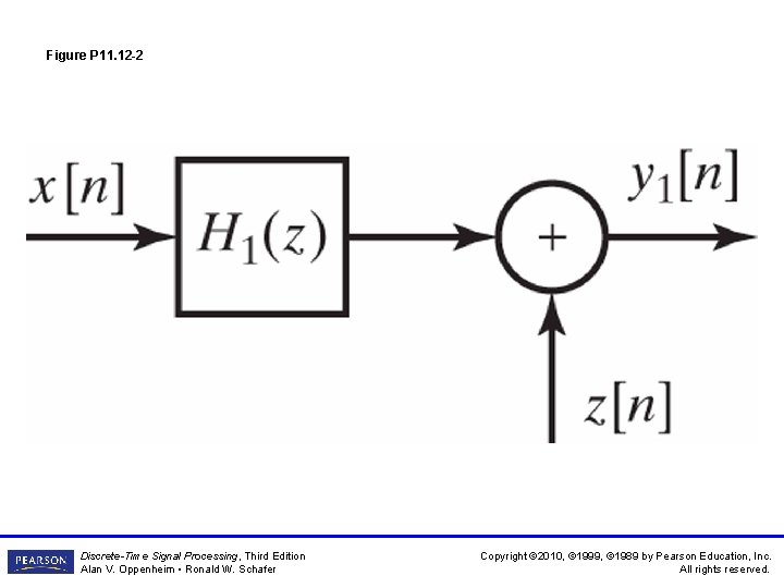
Figure P 11. 12 -2 Discrete-Time Signal Processing, Third Edition Alan V. Oppenheim • Ronald W. Schafer Copyright © 2010, © 1999, © 1989 by Pearson Education, Inc. All rights reserved.

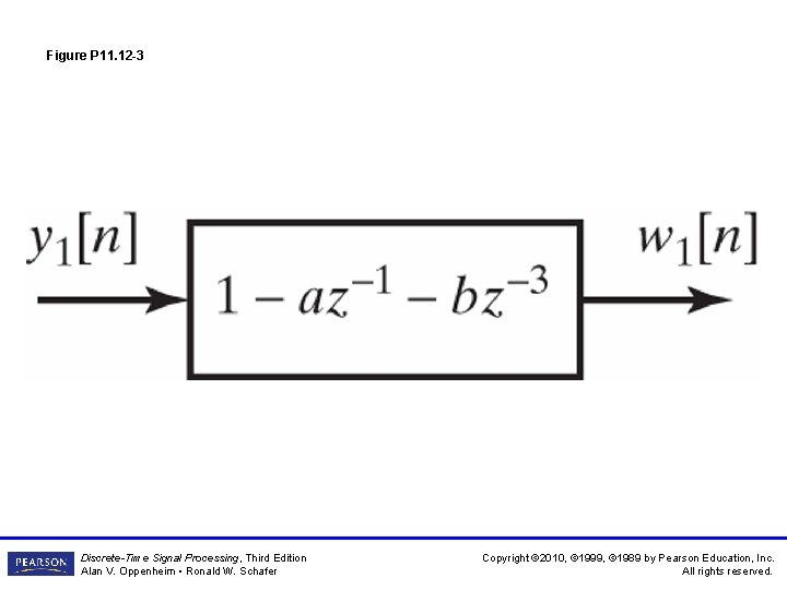
Figure P 11. 12 -3 Discrete-Time Signal Processing, Third Edition Alan V. Oppenheim • Ronald W. Schafer Copyright © 2010, © 1999, © 1989 by Pearson Education, Inc. All rights reserved.

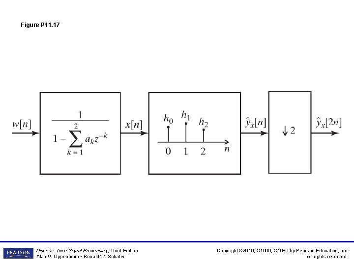
Figure P 11. 17 Discrete-Time Signal Processing, Third Edition Alan V. Oppenheim • Ronald W. Schafer Copyright © 2010, © 1999, © 1989 by Pearson Education, Inc. All rights reserved.

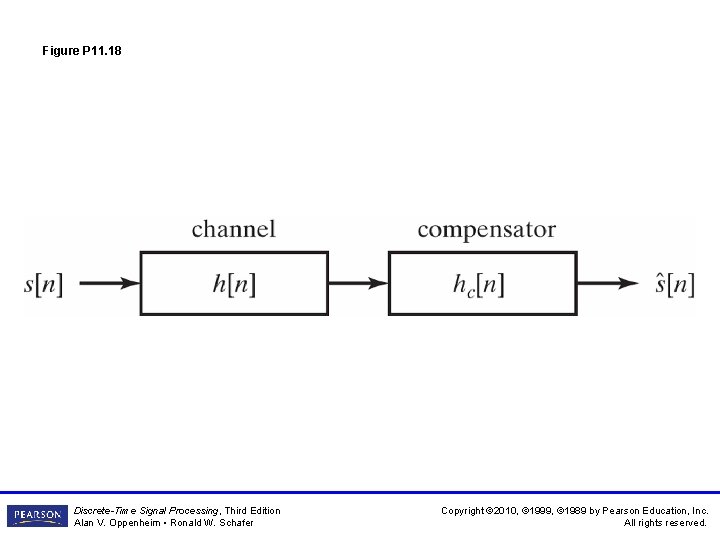
Figure P 11. 18 Discrete-Time Signal Processing, Third Edition Alan V. Oppenheim • Ronald W. Schafer Copyright © 2010, © 1999, © 1989 by Pearson Education, Inc. All rights reserved.

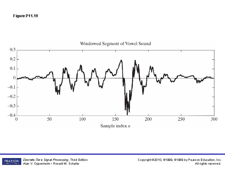
Figure P 11. 19 Discrete-Time Signal Processing, Third Edition Alan V. Oppenheim • Ronald W. Schafer Copyright © 2010, © 1999, © 1989 by Pearson Education, Inc. All rights reserved.

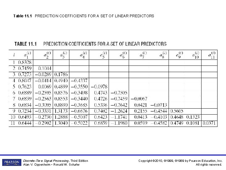
Table 11. 1 PREDICTION COEFFICIENTS FOR A SET OF LINEAR PREDICTORS Discrete-Time Signal Processing, Third Edition Alan V. Oppenheim • Ronald W. Schafer Copyright © 2010, © 1999, © 1989 by Pearson Education, Inc. All rights reserved.

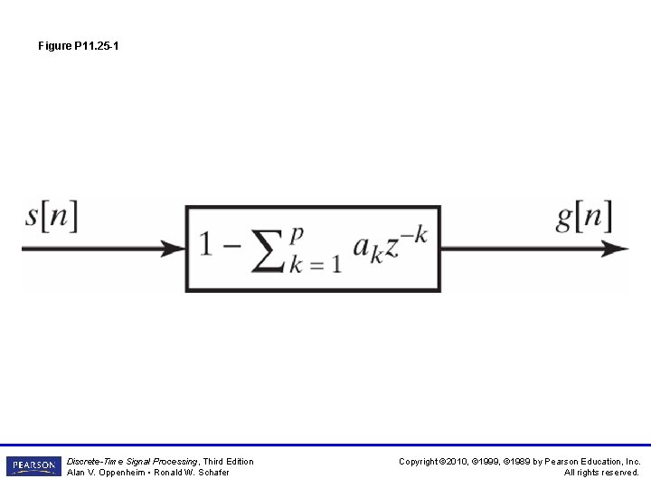
Figure P 11. 25 -1 Discrete-Time Signal Processing, Third Edition Alan V. Oppenheim • Ronald W. Schafer Copyright © 2010, © 1999, © 1989 by Pearson Education, Inc. All rights reserved.

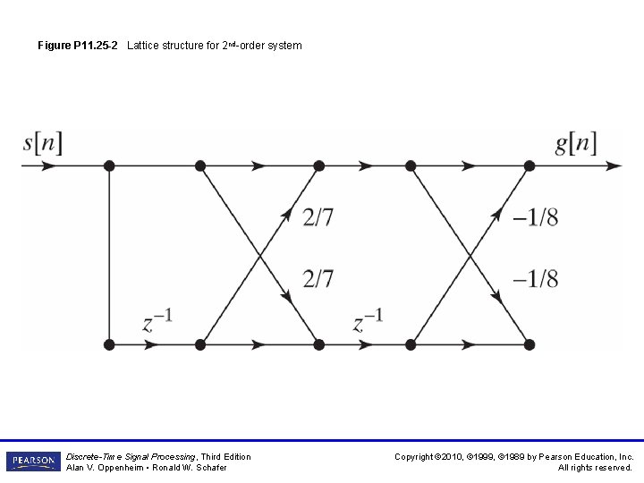
Figure P 11. 25 -2 Lattice structure for 2 nd-order system Discrete-Time Signal Processing, Third Edition Alan V. Oppenheim • Ronald W. Schafer Copyright © 2010, © 1999, © 1989 by Pearson Education, Inc. All rights reserved.

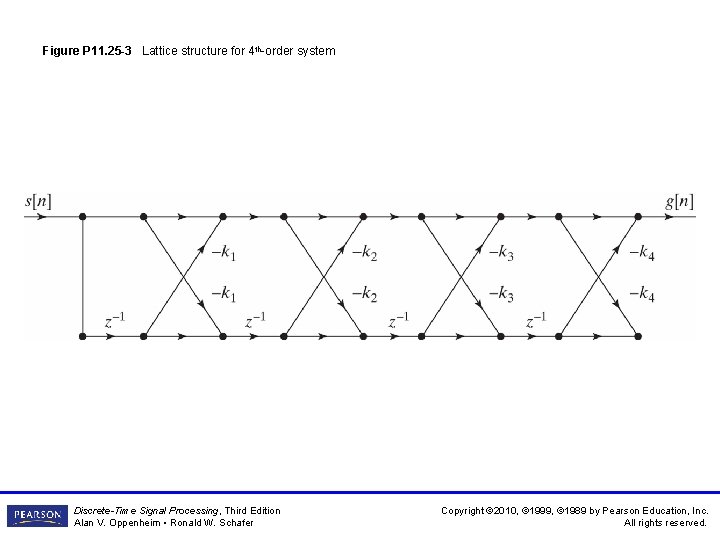
Figure P 11. 25 -3 Lattice structure for 4 th-order system Discrete-Time Signal Processing, Third Edition Alan V. Oppenheim • Ronald W. Schafer Copyright © 2010, © 1999, © 1989 by Pearson Education, Inc. All rights reserved.

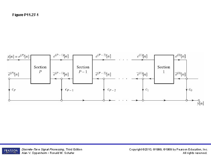
Figure P 11. 27 -1 Discrete-Time Signal Processing, Third Edition Alan V. Oppenheim • Ronald W. Schafer Copyright © 2010, © 1999, © 1989 by Pearson Education, Inc. All rights reserved.

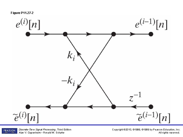
Figure P 11. 27 -2 Discrete-Time Signal Processing, Third Edition Alan V. Oppenheim • Ronald W. Schafer Copyright © 2010, © 1999, © 1989 by Pearson Education, Inc. All rights reserved.