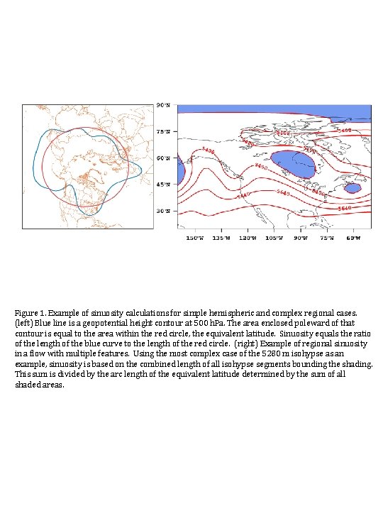
Figure 1 Example of sinuosity calculations for simple

Figure 1. Example of sinuosity calculations for simple hemispheric and complex regional cases. (left) Blue line is a geopotential height contour at 500 h. Pa. The area enclosed poleward of that contour is equal to the area within the red circle, the equivalent latitude. Sinuosity equals the ratio of the length of the blue curve to the length of the red circle. (right) Example of regional sinuosity in a flow with multiple features. Using the most complex case of the 5280 m isohypse as an example, sinuosity is based on the combined length of all isohypse segments bounding the shading. This sum is divided by the arc length of the equivalent latitude determined by the sum of all shaded areas.

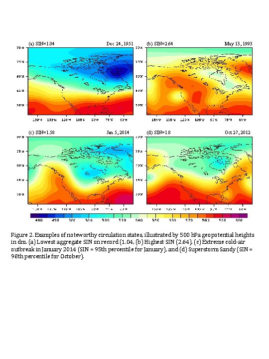
(a) SIN=1. 04 Dec 24, 1951 (b) SIN=2. 64 May 13, 1993 (c) SIN=1. 58 Jan 5, 2014 (d) SIN=1. 8 Oct 27, 2012 Figure 2. Examples of noteworthy circulation states, illustrated by 500 h. Pa geopotential heights in dm. (a) Lowest aggregate SIN on record (1. 04, (b) Highest SIN (2. 64), (c) Extreme cold-air outbreak in January 2014 (SIN = 95 th percentile for January), and (d) Superstorm Sandy (SIN = 98 th percentile for October).

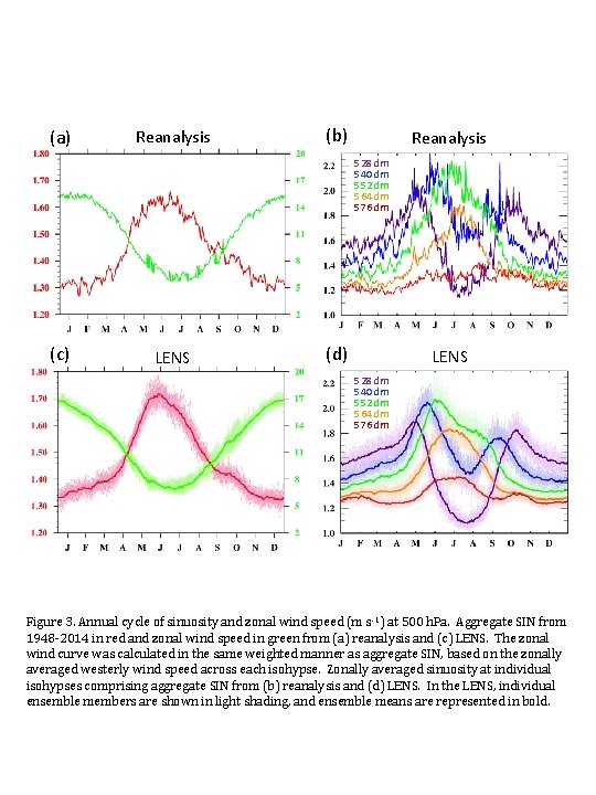
(a) Reanalysis (b) Reanalysis 528 dm 540 dm 552 dm 564 dm 576 dm (c) LENS (d) LENS 528 dm 540 dm 552 dm 564 dm 576 dm Figure 3. Annual cycle of sinuosity and zonal wind speed (m s -1) at 500 h. Pa. Aggregate SIN from 1948 -2014 in red and zonal wind speed in green from (a) reanalysis and (c) LENS. The zonal wind curve was calculated in the same weighted manner as aggregate SIN, based on the zonally averaged westerly wind speed across each isohypse. Zonally averaged sinuosity at individual isohypses comprising aggregate SIN from (b) reanalysis and (d) LENS. In the LENS, individual ensemble members are shown in light shading, and ensemble means are represented in bold.

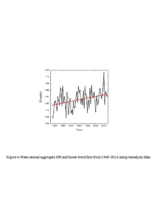
Figure 4. Mean annual aggregate SIN and linear trend line from 1948 -2014 using reanalysis data.

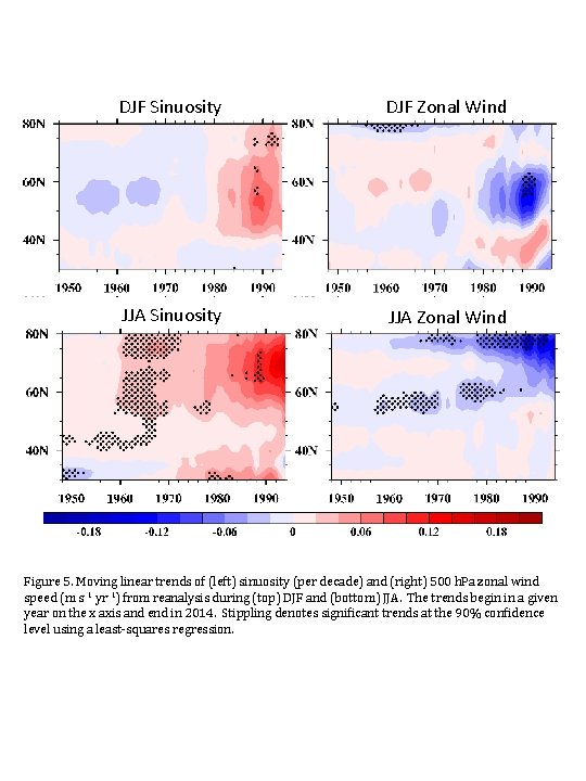
DJF Sinuosity DJF Zonal Wind JJA Sinuosity JJA Zonal Wind Figure 5. Moving linear trends of (left) sinuosity (per decade) and (right) 500 h. Pa zonal wind speed (m s-1 yr-1) from reanalysis during (top) DJF and (bottom) JJA. The trends begin in a given year on the x axis and end in 2014. Stippling denotes significant trends at the 90% confidence level using a least-squares regression.

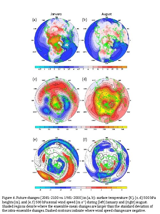
January August (a) (b) (c) (d) (e) (f) Figure 6. Future changes (2081 -2100 vs. 1981 -2000) in (a, b): surface temperature (K), (c, d) 500 h. Pa heights (m), and (e, f) 500 h. Pa zonal wind speed (m s-1) during (left) January and (right) August. Shaded regions denote where the ensemble-mean changes are larger than the standard deviation of the intra-ensemble changes. Dashed contours indicate where wind speed changes are negative.

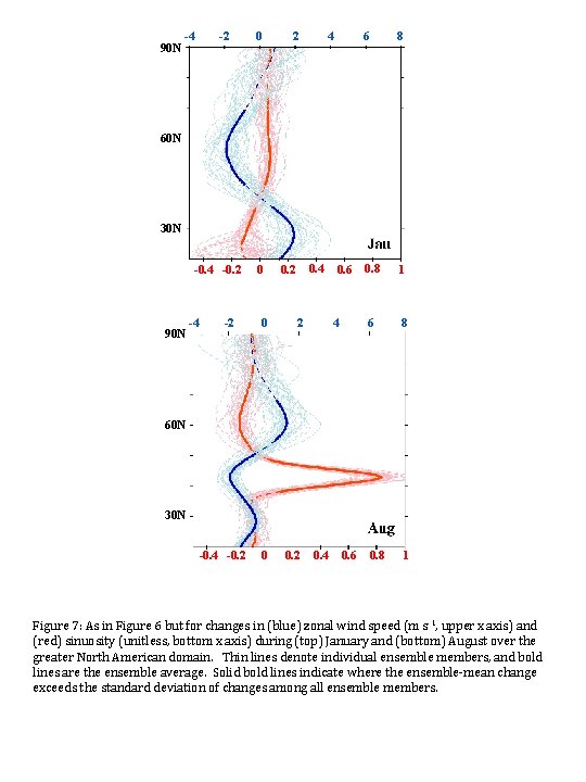
90 N -4 -2 0 0. 2 4 6 8 0. 8 1 60 N 30 N -0. 4 -0. 2 90 N -4 -2 0. 4 0 2 0 0. 2 0. 6 4 6 8 0. 8 1 60 N 30 N -0. 4 -0. 2 0. 4 0. 6 Figure 7: As in Figure 6 but for changes in (blue) zonal wind speed (m s-1, upper x axis) and (red) sinuosity (unitless, bottom x axis) during (top) January and (bottom) August over the greater North American domain. Thin lines denote individual ensemble members, and bold lines are the ensemble average. Solid bold lines indicate where the ensemble-mean change exceeds the standard deviation of changes among all ensemble members.

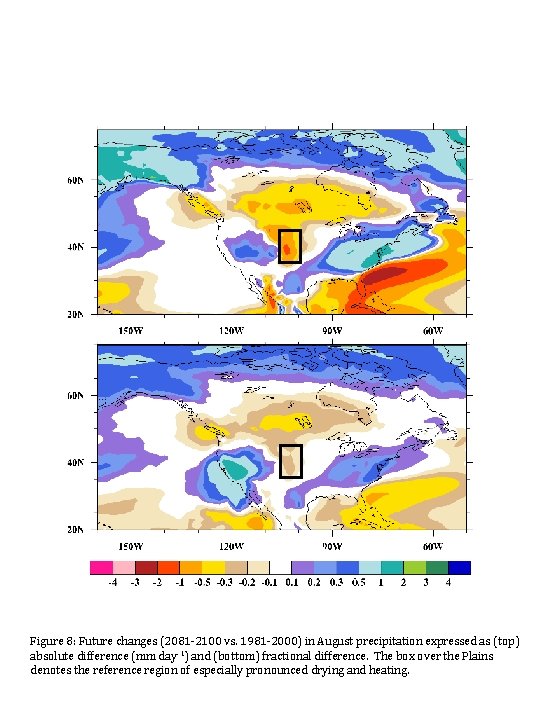
Figure 8: Future changes (2081 -2100 vs. 1981 -2000) in August precipitation expressed as (top) absolute difference (mm day-1) and (bottom) fractional difference. The box over the Plains denotes the reference region of especially pronounced drying and heating.

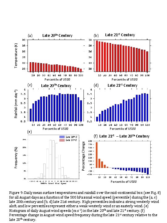
Late 20 th Century (b) Late 21 st Century Temperature (K) (a) Percentile of U 500 Late 20 th Century (d) Late 21 st Century Rainfall (mm day-1) (c) Percentile of U 500 (e) Percentile of U 500 (f) Late 21 st – Late 20 th Century Percentage Change Frequency (%) Late 20 th C Late 21 st C Percentile of U 500 Figure 9: Daily mean surface temperatures and rainfall over the mid-continental box (see Fig. 8) for all August days as a function of the 500 h. Pa zonal wind speed (percentile) during the (a, c) late 20 th century and (b, d) late 21 st century. High percentiles indicate a strong westerly wind aloft, and low percentiles represent either a weak westerly wind or an easterly wind. (e) Histogram of daily August wind speeds (m s-1) in the late 20 th and late 21 st century. (f) Percentage change in August wind speed frequency during the late 21 st century relative to the late 20 th century.

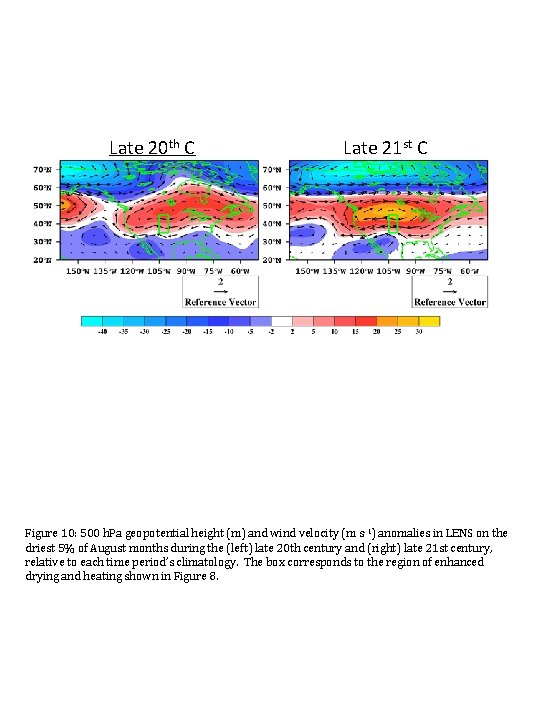
Late 20 th C Late 21 st C Figure 10: 500 h. Pa geopotential height (m) and wind velocity (m s-1) anomalies in LENS on the driest 5% of August months during the (left) late 20 th century and (right) late 21 st century, relative to each time period’s climatology. The box corresponds to the region of enhanced drying and heating shown in Figure 8.

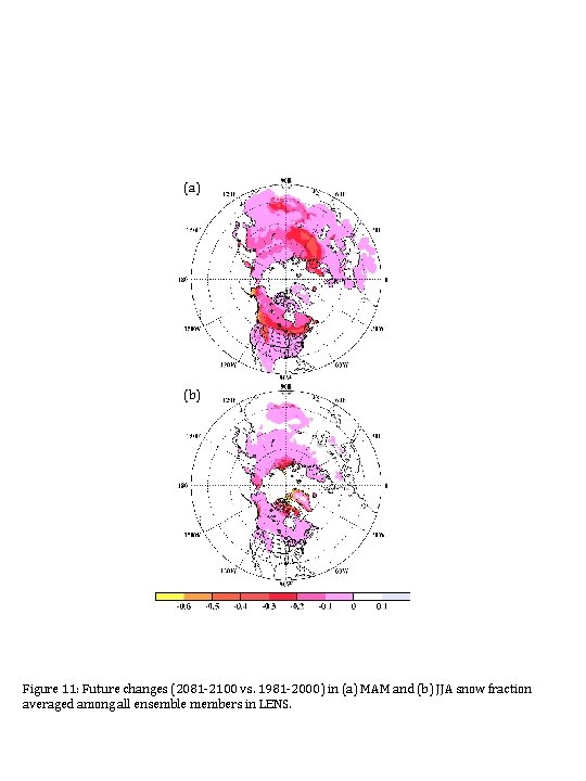
(a) (b) Figure 11: Future changes (2081 -2100 vs. 1981 -2000) in (a) MAM and (b) JJA snow fraction averaged among all ensemble members in LENS.

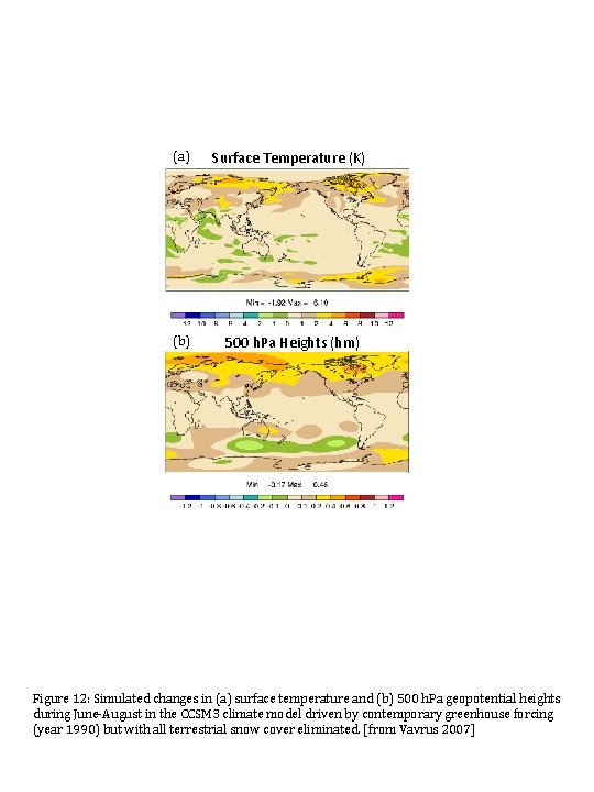
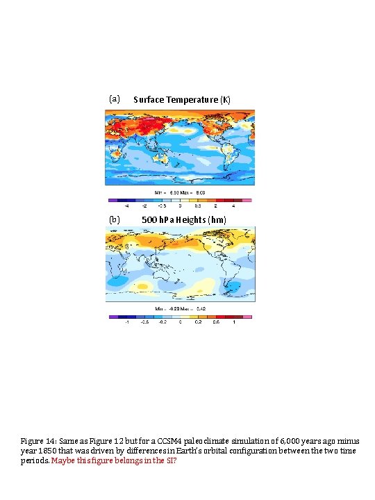
(a) Surface Temperature (K) (b) 500 h. Pa Heights (hm) Figure 12: Simulated changes in (a) surface temperature and (b) 500 h. Pa geopotential heights during June-August in the CCSM 3 climate model driven by contemporary greenhouse forcing (year 1990) but with all terrestrial snow cover eliminated. [from Vavrus 2007]

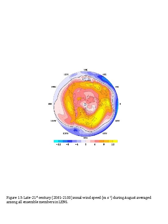
Figure 13: Late-21 st century (2081 -2100) zonal wind speed (m s-1) during August averaged among all ensemble members in LENS.

(a) Surface Temperature (K) (b) 500 h. Pa Heights (hm) Figure 14: Same as Figure 12 but for a CCSM 4 paleoclimate simulation of 6, 000 years ago minus year 1850 that was driven by differences in Earth’s orbital configuration between the two time periods. Maybe this figure belongs in the SI?