FFT Convolution Michael Phipps Vallary S Bhopatkar Convolution

FFT Convolution Michael Phipps Vallary S. Bhopatkar
 and g(t) are two functions and")
Convolution theorem �Convolution theorem for continuous case: �h(t) and g(t) are two functions and H(f) and G(f) are their corresponding Fourier Transform, then convolution is defined as Where g*h is in time domain and then convolution theorem is given by g*h ↔ G(f) H(f) Fourier transform of the convolution is just the product of the individual Fourier transform

� Convolution of two function is equal to their convolution in opposite order s*r =r*s � If s(t) is function represents signal then r(t) is response function and their convolution smears the signal s(t) in time according to response function r(t)
 is represented by its sampled values at equal time")
�Discrete case: �If signal s(t) is represented by its sampled values at equal time interval sj , rk is discrete set of numbers corresponds to response function then rk tells what multiple of the input signal is copied into identical output channel. �Therefore, the discrete convolution with response function of finite duration M is given by �If response function is non-zero in some range where M is very large even integer, then response function is called as finite impulse response (FIR)

The discrete convolution theorem �If signal sj is periodic with period N, then its discrete convolution with response function of finite duration N is member of the discrete Fourier transform pair

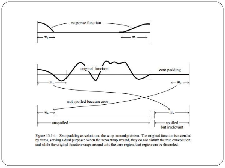
Zero Padding �Discrete convolution considered two assumptions: 1. Input signal is periodic 2. Duration of response function is same as the period of the data i. e. N � To work on these two constrains, zero padding method is used. � For response function M which shorter than N, can be expanded to length N by padding it with zeros. � i. e. define rk = 0 for M/2 ≤ k ≤ N/2 and also for –N/2 + 1 ≤ ≤ -M/2 +1
0 with some wrapped- around data")
�The first assumption pollute the first output channel (s*r)0 with some wrapped- around data from the far end �To make this pollution zero, we nee to set the buffer zone of zero padded values at the end of the sj vector. �Number of zero should be equal to most negative index for which the response function is non zero.

Use of FFT for convolution �After considering the zero padding for real data, the discrete convolution can be calculated using FFT algorithm. �First compute the discrete Fourier transform of s and r, and then multiply these two transform component by component �Take inverse discrete FT of the product in order to get convolution r*s

Deconvolution �This is a process of undoing smearing in a data set that has occurred under the influence of known response function �Now left hand side is know for deconvolution �In order to get transform of deconvolution signal, will divide transform of known convolution by the transform of response function

Drawbacks of this method �It can go mathematically wrong if response function has zero value �It is sensitive to the noise in the input data and the to the accuracy of the response function

Convolving or deconvolving very large data set �If the data set is very large, we can break it up into small section and convolve each section separately �This method cause wraparound effect at the end and to overcome this problem, there are two solutions: 1. Overlap-save method 2. Overlap-add method

� 1. Overlap-save method �Pad only beginning of the data with zeros to avoid wraparound pollution �Convolve the section and throw out the points at each end that are polluted �Choose next section such that the first points should overlap the last points of the preceding section �It should overlap in such away that the end of section should recomputed as first section of unpolluted output points of subsequent section

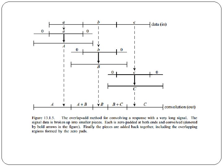
� 2. Overlap-add method: �In this method, distinct sections are considered and zero pad it from the both ends �Take convolution of each section and then overlap and add these sections outputs �Therefore, output points near end of one section will have response due to the input points at the beginning of the next section and data is added properly.

Resources �Numerical recipes
- Slides: 16