Feynman diagrams In 1940 s R Feynman developed

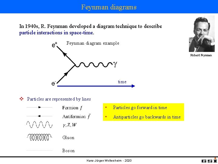
Feynman diagrams In 1940 s, R. Feynman developed a diagram technique to describe particle interactions in space-time. Feynman diagram example Richard Feynman time v Particles are represented by lines • Particles go forward in time • Antiparticles go backwards in time Gluon Boson Hans-Jürgen Wollersheim - 2020

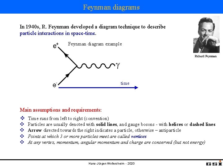
Feynman diagrams In 1940 s, R. Feynman developed a diagram technique to describe particle interactions in space-time. Feynman diagram example Richard Feynman time Main assumptions and requirements: v Time runs from left to right (convention) v v Particles are usually denoted with solid lines, and gauge bosons - with helices or dashed lines Arrow directed towards the right indicates a particle, otherwise – antiparticle Points at which 3 or more particles meet are called vertices At any vertex, momentum, angular momentum and charge are conserved (but not energy) Hans-Jürgen Wollersheim - 2020

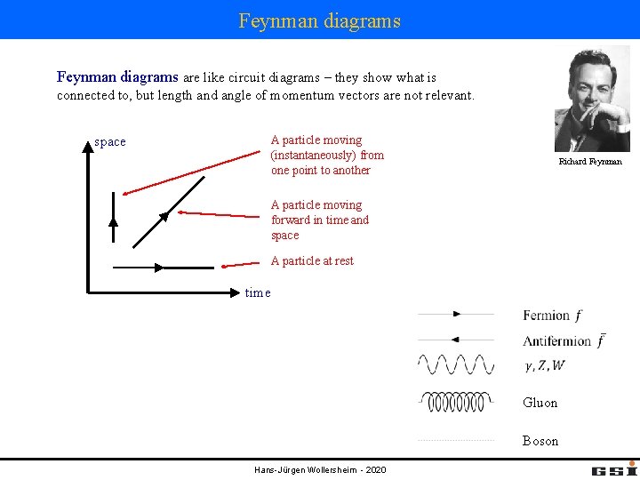
Feynman diagrams are like circuit diagrams – they show what is connected to, but length and angle of momentum vectors are not relevant. space A particle moving (instantaneously) from one point to another Richard Feynman A particle moving forward in time and space A particle at rest time Gluon Boson Hans-Jürgen Wollersheim - 2020

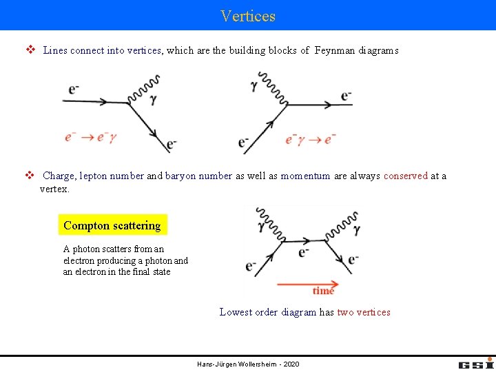
Vertices v Lines connect into vertices, which are the building blocks of Feynman diagrams v Charge, lepton number and baryon number as well as momentum are always conserved at a vertex. Compton scattering A photon scatters from an electron producing a photon and an electron in the final state Lowest order diagram has two vertices Hans-Jürgen Wollersheim - 2020

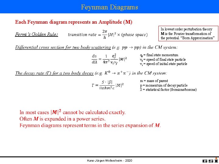
Feynman Diagrams Each Feynman diagram represents an Amplitude (M) In lowest order perturbation theory M is the Fourier transformation of the potential. “Born Approximation” Fermi’s Golden Rule: qf = final state momentum vf = speed of final state particle vi = speed of initial state particle m = mass of parent p = momentum of decay particle S = statistical factor (fermions/bosons) Hans-Jürgen Wollersheim - 2020

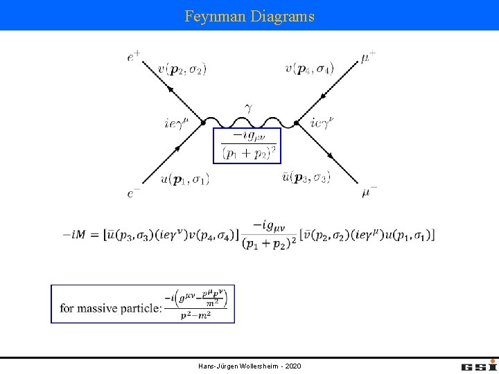
Feynman Diagrams Hans-Jürgen Wollersheim - 2020

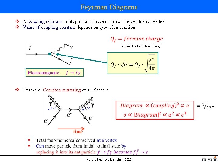
Feynman Diagrams v A coupling constant (multiplication factor) is associated with each vertex. v Value of coupling constant depends on type of interaction (in units of electron charge) v Example: Compton scattering of an electron Hans-Jürgen Wollersheim - 2020

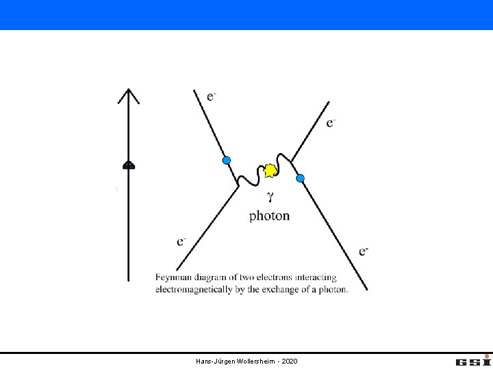
Hans-Jürgen Wollersheim - 2020

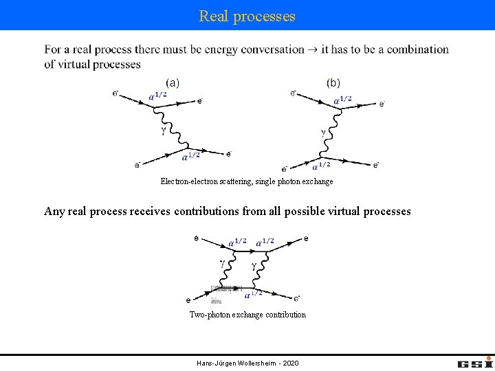
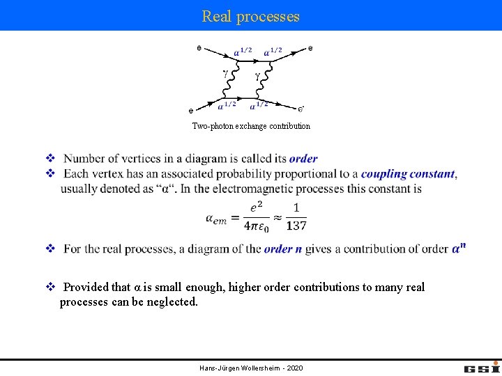
Real processes Electron-electron scattering, single photon exchange Any real process receives contributions from all possible virtual processes Two-photon exchange contribution Hans-Jürgen Wollersheim - 2020

Real processes Two-photon exchange contribution v Provided that α is small enough, higher order contributions to many real processes can be neglected. Hans-Jürgen Wollersheim - 2020

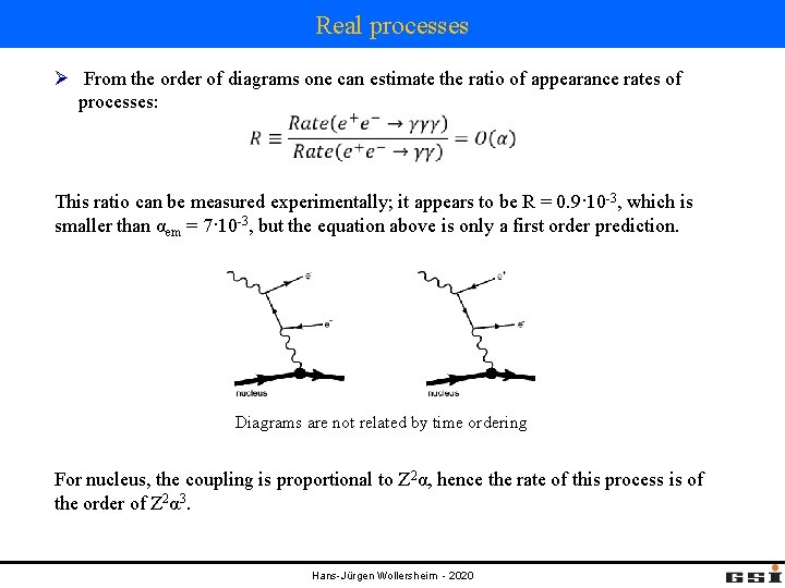
Real processes Ø From the order of diagrams one can estimate the ratio of appearance rates of processes: This ratio can be measured experimentally; it appears to be R = 0. 9·10 -3, which is smaller than αem = 7·10 -3, but the equation above is only a first order prediction. Diagrams are not related by time ordering For nucleus, the coupling is proportional to Z 2α, hence the rate of this process is of the order of Z 2α 3. Hans-Jürgen Wollersheim - 2020

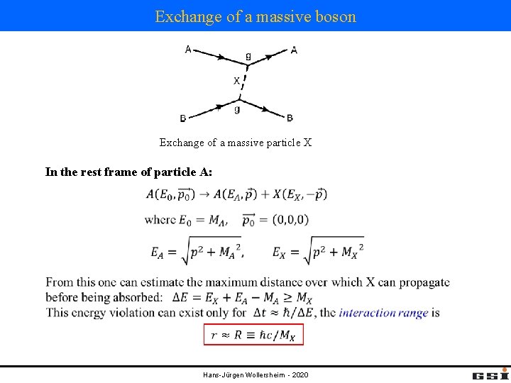
Exchange of a massive boson Exchange of a massive particle X In the rest frame of particle A: Hans-Jürgen Wollersheim - 2020

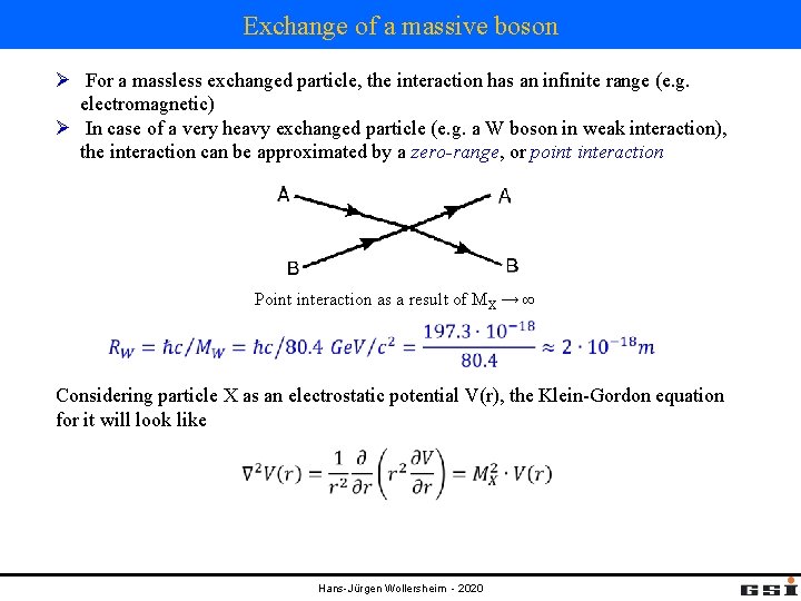
Exchange of a massive boson Ø For a massless exchanged particle, the interaction has an infinite range (e. g. electromagnetic) Ø In case of a very heavy exchanged particle (e. g. a W boson in weak interaction), the interaction can be approximated by a zero-range, or point interaction Point interaction as a result of MX → ∞ Considering particle X as an electrostatic potential V(r), the Klein-Gordon equation for it will look like Hans-Jürgen Wollersheim - 2020

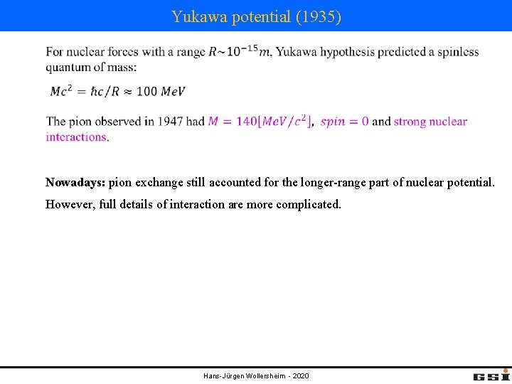
Yukawa potential (1935) Nowadays: pion exchange still accounted for the longer-range part of nuclear potential. However, full details of interaction are more complicated. Hans-Jürgen Wollersheim - 2020

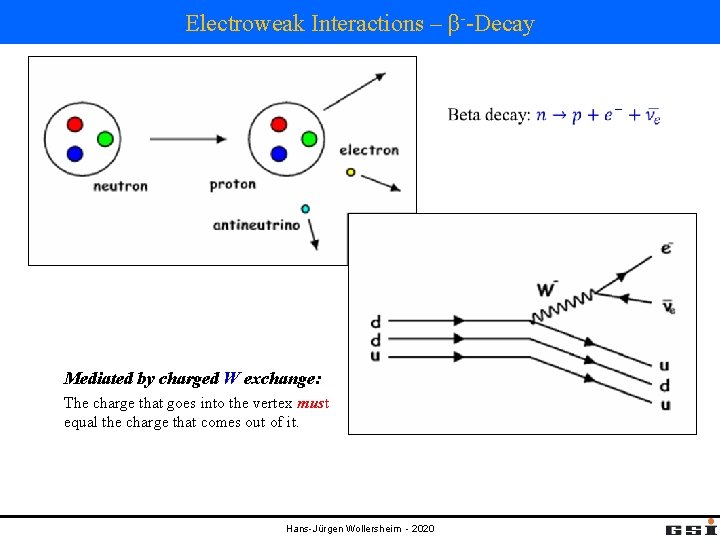
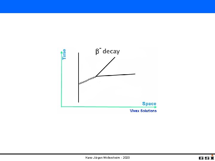
Electroweak Interactions – β--Decay Mediated by charged W exchange: The charge that goes into the vertex must equal the charge that comes out of it. Hans-Jürgen Wollersheim - 2020

Hans-Jürgen Wollersheim - 2020

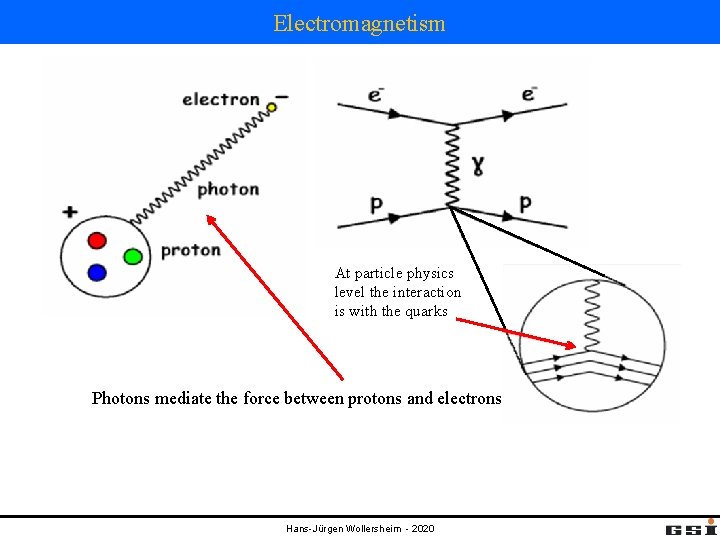
Electromagnetism At particle physics level the interaction is with the quarks Photons mediate the force between protons and electrons Hans-Jürgen Wollersheim - 2020

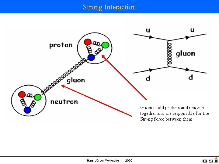
Strong Interaction Gluons hold protons and neutron together and are responsible for the Strong force between them Hans-Jürgen Wollersheim - 2020

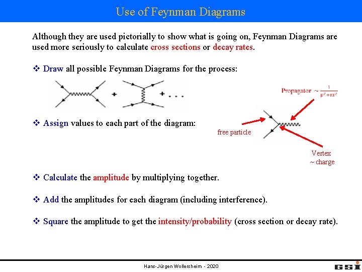
Use of Feynman Diagrams Although they are used pictorially to show what is going on, Feynman Diagrams are used more seriously to calculate cross sections or decay rates. v Draw all possible Feynman Diagrams for the process: v Assign values to each part of the diagram: free particle Vertex ~ charge v Calculate the amplitude by multiplying together. v Add the amplitudes for each diagram (including interference). v Square the amplitude to get the intensity/probability (cross section or decay rate). Hans-Jürgen Wollersheim - 2020