Feedback control theory An overview and connections to
Feedback control theory: An overview and connections to biochemical systems theory Sigurd Skogestad Department of Chemical Engineering Norwegian University of Science and Tecnology (NTNU) Trondheim, Norway VIIth International Symposium on Biochemical Systems Theory Averøy, Norway, 17 -20 June 2002 1
Motivation • I have co-authored a book: ”Multivariable feedback control – analysis and design” (Wiley, 1996) – What parts could be useful for systems biochemistry? • Control as a field is closely related to systems theory – The more general systems theory concepts are assumed known • Here: Focus on the use of negative feedback • Some other areas where control may contribute (Not covered): – Identification of dynamic models from data (not in my book anyway) – Model reduction – Nonlinear control (also not in my book) 2
Outline 1. Introduction: Feedforward and negative feedback control 2. Introductory examples – Feedback is an extremely powerful tool (BUT: So simple that it is frequently overlooked) 3. Control theory and possible contributions 4. Fundamental limitation on negative feedback control 5. Cascade control and control of complex large-scale engineering system • Hierarchy (cascades) of single-input-single-output (SISO) control loops 6. Design of hierarchical control systems • • • Overall operational objectives Which variable to control (primary output) ? Self-optimizing control 7. Summary and concluding remarks 3
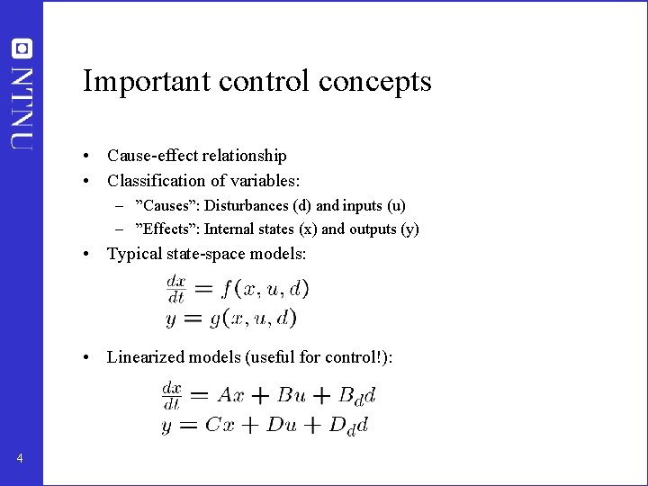
Important control concepts • Cause-effect relationship • Classification of variables: – ”Causes”: Disturbances (d) and inputs (u) – ”Effects”: Internal states (x) and outputs (y) • Typical state-space models: • Linearized models (useful for control!): 4
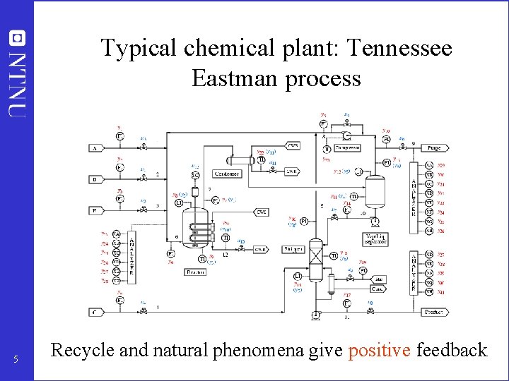
Typical chemical plant: Tennessee Eastman process 5 Recycle and natural phenomena give positive feedback
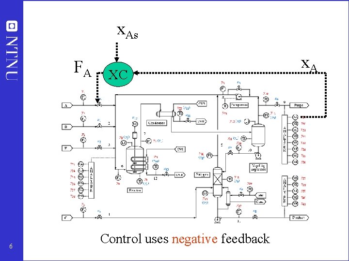
x. As FA 6 XC Control uses negative feedback x. A
Control • Active adjustment of inputs (available degrees of freedom, u) to achieve the operational objectives of the system • Most cases: Acceptable operation = ”Output (y) close to desired setpoint (ys)” 7
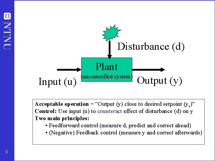
Disturbance (d) Plant Input (u) (uncontrolled system) Output (y) Acceptable operation = ”Output (y) close to desired setpoint (ys)” Control: Use input (u) to counteract effect of disturbance (d) on y Two main principles: • Feedforward control (measure d, predict and correct ahead) • (Negative) Feedback control (measure y and correct afterwards) 8
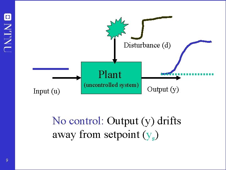
Disturbance (d) Plant Input (u) (uncontrolled system) Output (y) No control: Output (y) drifts away from setpoint (ys) 9
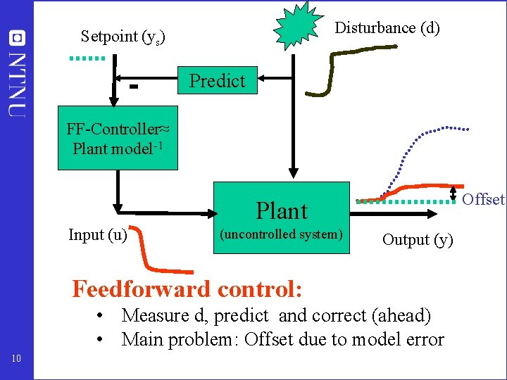
Disturbance (d) Setpoint (ys) Predict FF-Controller≈ Plant model-1 Offset Plant Input (u) (uncontrolled system) Output (y) Feedforward control: • Measure d, predict and correct (ahead) • Main problem: Offset due to model error 10
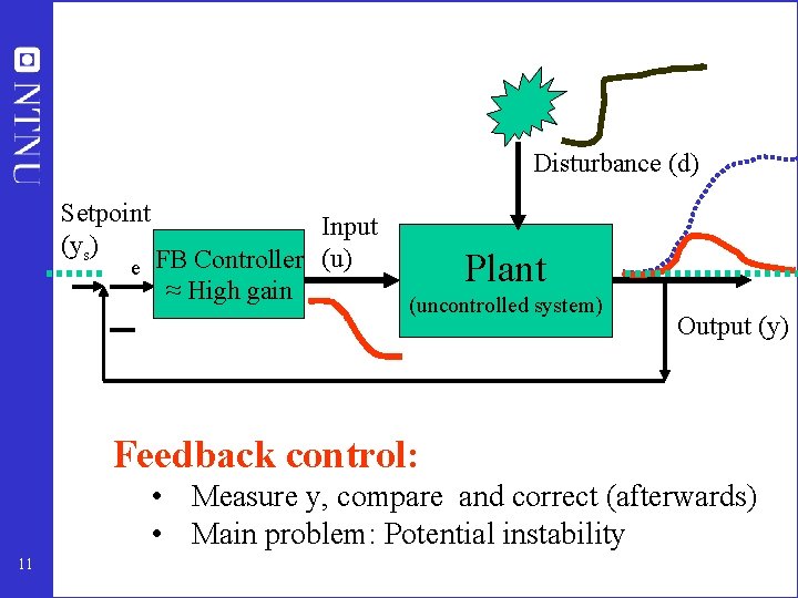
Disturbance (d) Setpoint (ys) Input e FB Controller (u) ≈ High gain Plant (uncontrolled system) Output (y) Feedback control: • Measure y, compare and correct (afterwards) • Main problem: Potential instability 11
Outline 1. Introduction: Feedforward and feedback control 2. Introductory examples – (Negative) Feedback is an extremely powerful tool (BUT: So simple that it is frequently overlooked) 3. Control theory and possible contributions 4. Fundamental limitation on control 5. Cascade control and control of complex large-scale engineering system • Hierarchy (cascades) of single-input-single-output (SISO) control loops 6. Design of hierarchical control systems • • • Overall operational objectives Which variable to control (primary output) ? Self-optimizing control 7. Summary and concluding remarks 12
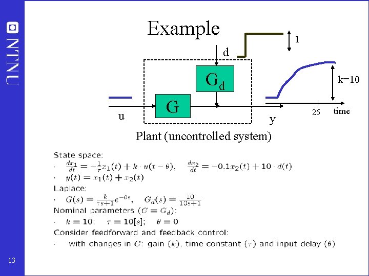
Example 1 d Gd u 13 G y Plant (uncontrolled system) k=10 25 time
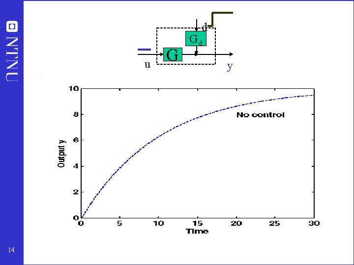
d u 14 G Gd y
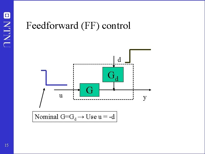
Feedforward (FF) control d Gd u G Nominal G=Gd → Use u = -d 15 y
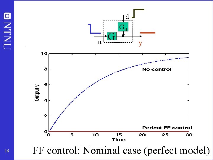
d u 16 G Gd y FF control: Nominal case (perfect model)
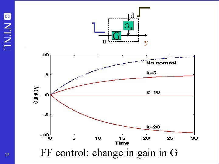
d u 17 G Gd y FF control: change in gain in G
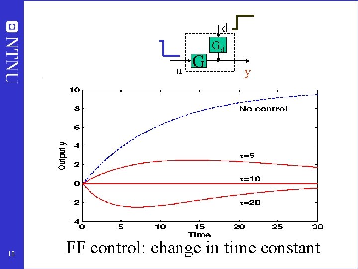
d u 18 G Gd y FF control: change in time constant
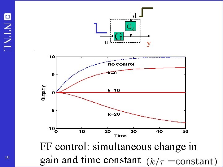
d u 19 G Gd y FF control: simultaneous change in gain and time constant
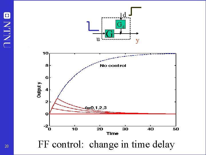
d u 20 G Gd y FF control: change in time delay
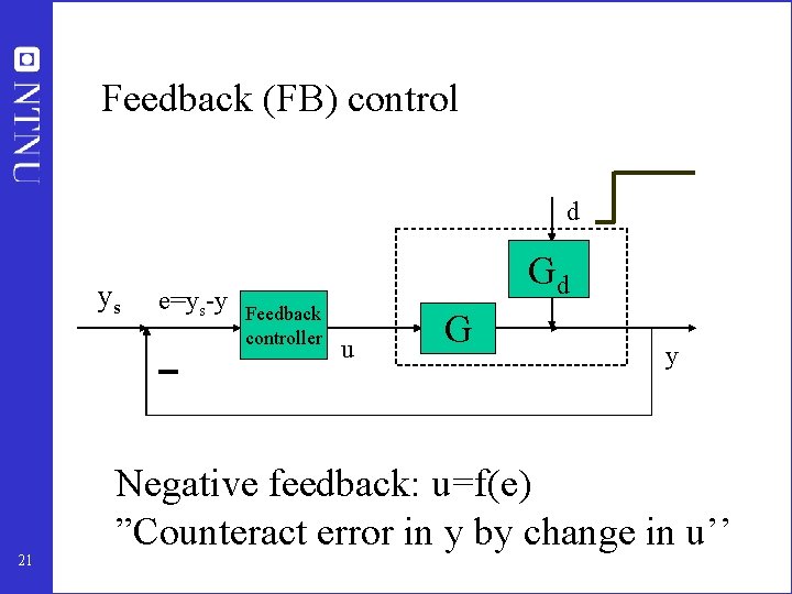
Feedback (FB) control d ys 21 e=ys-y Gd Feedback controller u G y Negative feedback: u=f(e) ”Counteract error in y by change in u’’
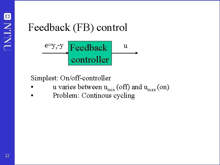
Feedback (FB) control e=ys-y Feedback controller u Simplest: On/off-controller • u varies between umin (off) and umax (on) • Problem: Continous cycling 22
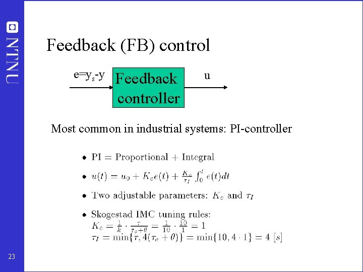
Feedback (FB) control e=ys-y Feedback controller u Most common in industrial systems: PI-controller 23
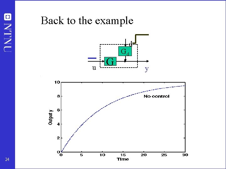
Back to the example d u 24 G Gd y
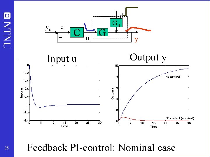
d ys e C Input u 25 u G Gd y Output y Feedback PI-control: Nominal case
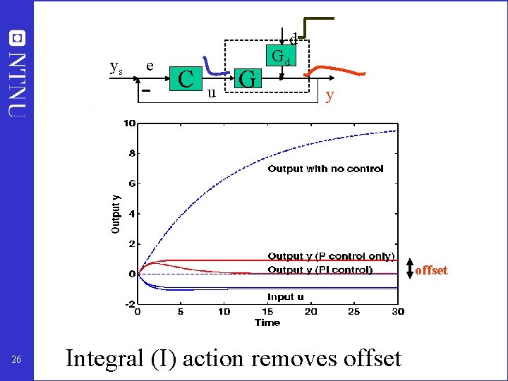
d ys e C u G Gd y offset 26 Integral (I) action removes offset
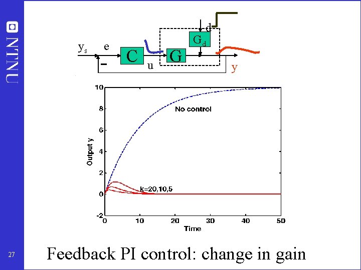
d ys 27 e C u G Gd y Feedback PI control: change in gain
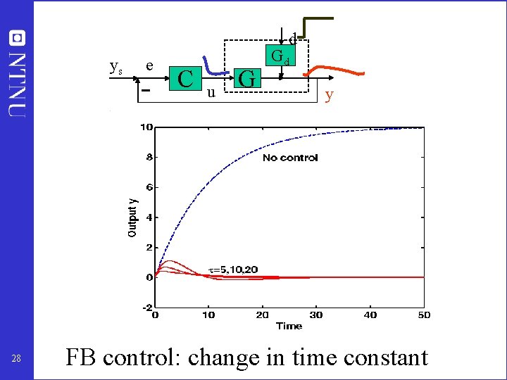
d ys 28 e C u G Gd y FB control: change in time constant
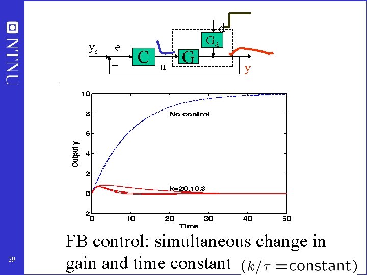
d ys 29 e C u G Gd y FB control: simultaneous change in gain and time constant
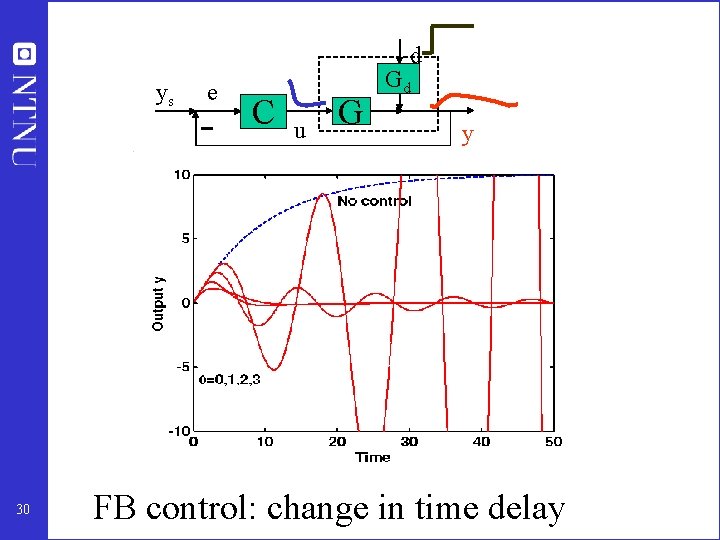
d ys 30 e C u G Gd y FB control: change in time delay
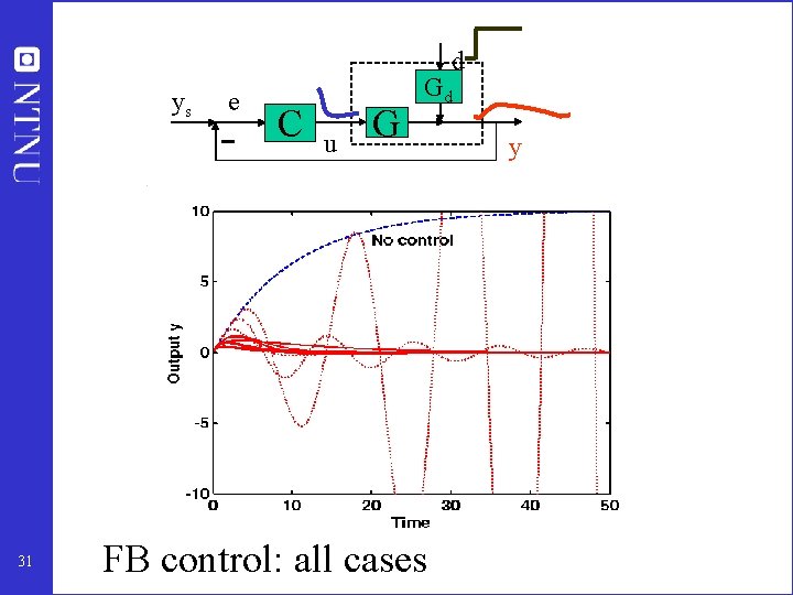
d ys 31 e C u G Gd FB control: all cases y
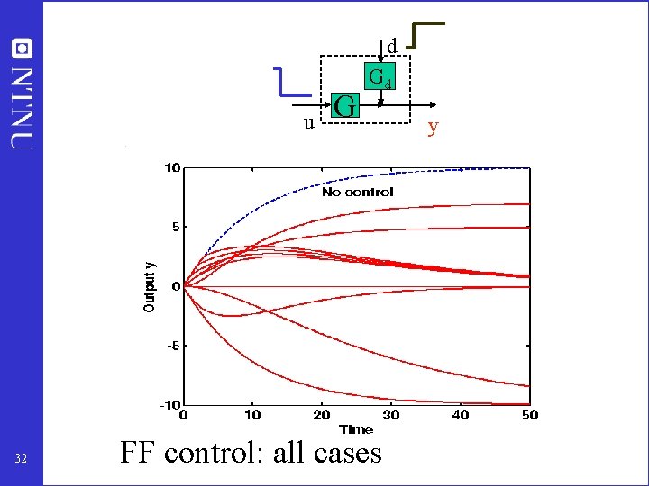
d u 32 G Gd FF control: all cases y
Summary example • Feedforward control is NOT ROBUST (it is sensitive to plant changes, e. g. in gain and time constant) • Feedforward control: gradual performance degradation • Feedback control is ROBUST (it is insensitive to plant changes, e. g. in gain and time constant) • Feedback control: sudden performance degradation (instability) Instability occurs if we over-react (loop gain is too large compared to effective time delay). • Feedback control: Changes system dynamics (eigenvalues) • Example was for single input - single output (SISO) case • Differences may be more striking in multivariable (MIMO) case 33
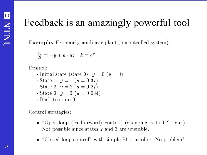
Feedback is an amazingly powerful tool 34
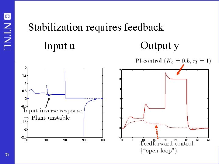
Stabilization requires feedback Input u 35 Output y
Why feedback? (and not feedforward control) • • Counteract unmeasured disturbances Reduce effect of changes / uncertainty (robustness) Change system dynamics (including stabilization) No explicit model required • MAIN PROBLEM • Potential instability (may occur suddenly) 36
Outline 1. Introduction: Feedforward and feedback control 2. Introductory examples – Feedback is an extremely powerful tool (BUT: So simple that it is frequently overlooked) 3. Control theory and possible contributions 4. Fundamental limitation on control 5. Cascade control and control of complex large-scale engineering system • Hierarchy (cascades) of single-input-single-output (SISO) control loops 6. Design of hierarchical control systems • • • Overall operational objectives Which variable to control (primary output) ? Self-optimizing control 7. Summary and concluding remarks 37
Overview of Control theory • Classical feedback control (1930 -1960) (Bode): – Single-loop (SISO) feedback control – Transfer functions, Frequency analysis (Bode-plot) – Fundamental feedback limitations (waterbed). Focus on robustness • Optimal control (1960 -1980) (Kalman): – Optimal design of Multivariable (MIMO) controllers – Model-based ”feedforward” thinking; no robustness guarantees (LQG) – State-space; Advanced mathematical tools (LQG) • Robust control (1980 -2000) (Zames, Doyle) – Combine classical and optimal control – Optimal design of controllers with guaranteed robustness (H∞) • Nonlinear control (1950 - ) – • 38 ”Feedforward thinking”, Mechanical systems Adaptive control (1970 -1985) (Åstrøm)
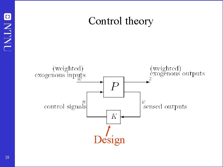
Control theory Design 39
Relationship to system biochemistry/biology: What can the control field contribute? • Advanced methods for model-based centralized controller design – Probably of minor interest in biological systems – Unlikely that nature has developed many multivariable control solutions • Understanding of feedback systems – Same inherent limitations apply in biological systems • Understanding and design of hierarchical control systems – Important both in engineering and biological systems – BUT: Underdeveloped area in control • ”Large scale systems community”: Out of touch with reality 40
Outline 1. Introduction: Feedforward and feedback control 2. Introductory examples – Feedback is an extremely powerful tool (BUT: So simple that it is frequently overlooked) 3. Control theory and possible contributions 4. Fundamental limitation on control 5. Cascade control and control of complex large-scale engineering system • Hierarchy (cascades) of single-input-single-output (SISO) control loops 6. Design of hierarchical control systems • • • Overall operational objectives Which variable to control (primary output) ? Self-optimizing control 7. Summary and concluding remarks 41
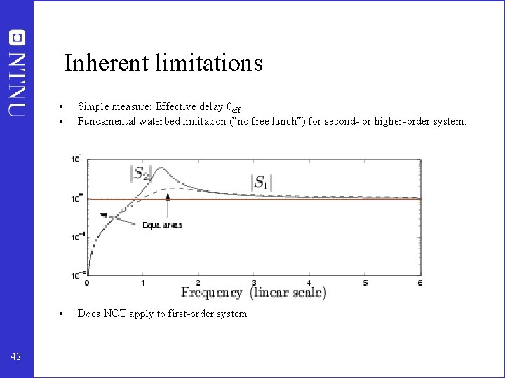
Inherent limitations 42 • • Simple measure: Effective delay θeff Fundamental waterbed limitation (”no free lunch”) for second- or higher-order system: • Does NOT apply to first-order system
Inherent limitations in plant (underlying uncontrolled system) • Effective delay: Includes inverse response, high-order dynamics • Multivariable systems: RHP-zeros (unstable inverse) – generalization of inverse response • Unstable plant. Not a problem in itself, but – Requires the active use of plant inputs – Requires that we can react sufficiently fast • ”Large” disturbances are a problem when combined with – Large effective delay: Cannot react sufficiently fast – Instability: Inputs may saturate and system goes unstable • All these may be quantified: For exampe, see my book 43
Outline 1. Introduction: Feedforward and feedback control 2. Introductory examples – Feedback is an extremely powerful tool (BUT: So simple that it is frequently overlooked) 3. Control theory and possible contributions 4. Fundamental limitation on control 5. Cascade control and control of complex large-scale engineering systems • Hierarchy (cascades) of single-input-single-output (SISO) control loops 6. Design of hierarchical control systems • • • Overall operational objectives Which variable to control (primary output) ? Self-optimizing control 7. Summary and concluding remarks 44
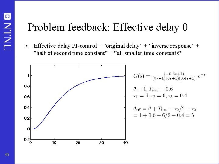
Problem feedback: Effective delay θ • Effective delay PI-control = ”original delay” + ”inverse response” + ”half of second time constant” + ”all smaller time constants” 45
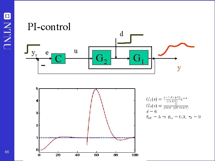
PI-control ys 46 e C d u G 2 G 1 y
Improve control? • Feedback: Some improvement possible with more complex controller – – For example, add derivative action (PID-controller) May reduce θeff from 5 s to 2 s Problem: Sensitive to measurement noise Does not remove the fundamental limitation (recall waterbed) • Feedforward: Good for time delay systems, but need model + measurement of disturbance. • Feedback: Add extra measurement and introduce local control – May remove the fundamental waterbed limitation • Waterbed limitation does not apply to first-order system – Cascade 47
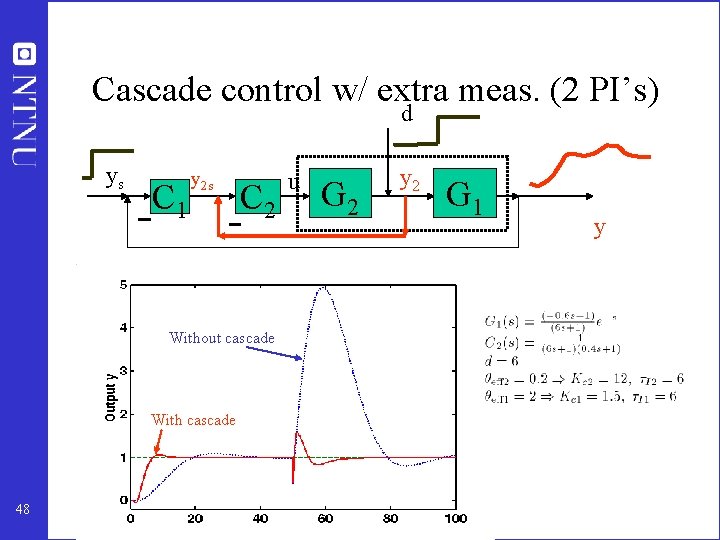
Cascade control w/ extra meas. (2 PI’s) d ys C 1 y 2 s C 2 Without cascade With cascade 48 u G 2 y 2 G 1 y
Cascade control • Inner fast (secondary) loop: – P or PI-control – Local disturbance rejection – Much smaller effective delay (0. 2 s) • Outer slower primary loop: – Reduced effective delay (2 s) • No loss in degrees of freedom – Setpoint in inner loop new degree of freedom • Time scale separation – • 49 Inner loop can be modelled as gain=1 + effective delay Very effective for control of large-scale systems
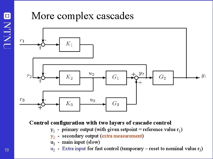
More complex cascades Control configuration with two layers of cascade control 50 y 1 y 2 u 3 u 2 - primary output (with given setpoint = reference value r 1) secondary output (extra measurement) main input (slow) Extra input for fast control (temporary – reset to nominal value r 3)
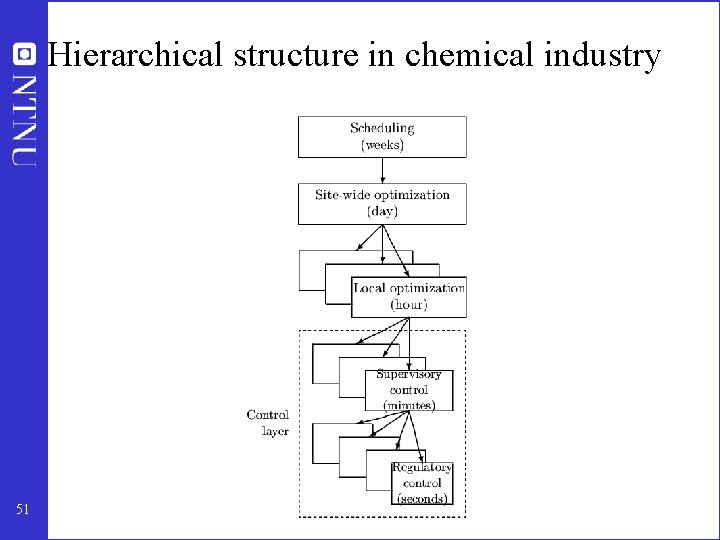
Hierarchical structure in chemical industry 51
Engineering systems • Most (all? ) large-scale engineering systems are controlled using hierarchies of quite simple single-loop controllers – Commercial aircraft – Large-scale chemical plant (refinery) • 1000’s of loops • Simple components: on-off + P-control + PI-control + nonlinear fixes + some feedforward Same in biological systems 52
Outline 1. Introduction: Feedforward and feedback control 2. Introductory examples – Feedback is an extremely powerful tool (BUT: So simple that it is frequently overlooked) 3. Control theory and possible contributions 4. Fundamental limitation on control 5. Cascade control and control of complex large-scale engineering system • Hierarchy (cascades) of single-input-single-output (SISO) control loops 6. Design of hierarchical control systems • • • Overall operational objectives Which variable to control (primary output) ? Self-optimizing control 7. Summary and concluding remarks 53
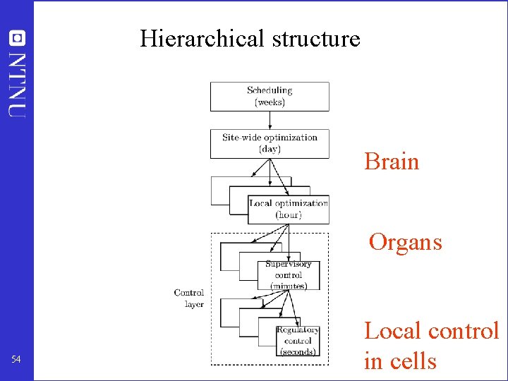
Hierarchical structure Brain Organs 54 Local control in cells
Alan Foss (“Critique of chemical process control theory”, AICh. E Journal, 1973): The central issue to be resolved. . . is the determination of control system structure. Which variables should be measured, which inputs should be manipulated and which links should be made between the two sets? 55
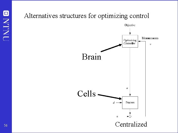
Alternatives structures for optimizing control What should we control? Brain Cells 56 Hierarchical Centralized
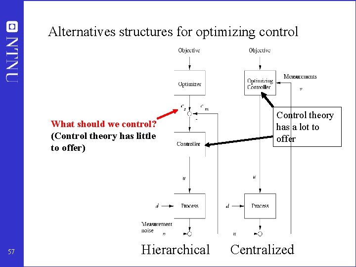
Alternatives structures for optimizing control What should we control? (Control theory has little to offer) 57 Hierarchical Control theory has a lot to offer Centralized
WHAT SHOULD WE CONTROL? Example: 10 km Run • Overall objective: Minimum time • No major disturbances • What should we control? – – constant speed? easy to measure with clock. constant heart beat? constant level of sugar? Constant level of lactic acid? Example: 10 km cross-country skiing • Overall objective: minimum time • Disturbance = hill. • What should we control? – Constant speed no longer optimal. – Could have a mix depending on disturbance (constant feed when flat, lactic acid in hill? , max speed downhill turn) Example: Cell • Overall objective = optimize cell growth? • What should we control? 58 – constant oxygen?
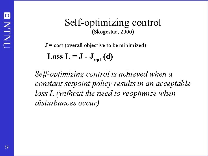
Self-optimizing control (Skogestad, 2000) J = cost (overall objective to be minimized) Loss L = J - Jopt (d) Self-optimizing control is achieved when a constant setpoint policy results in an acceptable loss L (without the need to reoptimize when disturbances occur) 59
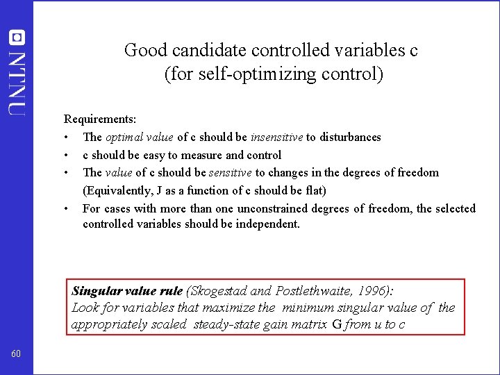
Good candidate controlled variables c (for self-optimizing control) Requirements: • The optimal value of c should be insensitive to disturbances • c should be easy to measure and control • The value of c should be sensitive to changes in the degrees of freedom (Equivalently, J as a function of c should be flat) • For cases with more than one unconstrained degrees of freedom, the selected controlled variables should be independent. Singular value rule (Skogestad and Postlethwaite, 1996): Look for variables that maximize the minimum singular value of the appropriately scaled steady-state gain matrix G from u to c 60
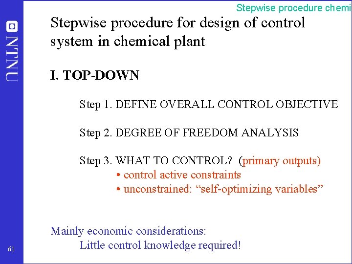
Stepwise procedure chemic Stepwise procedure for design of control system in chemical plant I. TOP-DOWN Step 1. DEFINE OVERALL CONTROL OBJECTIVE Step 2. DEGREE OF FREEDOM ANALYSIS Step 3. WHAT TO CONTROL? (primary outputs) • control active constraints • unconstrained: “self-optimizing variables” 61 Mainly economic considerations: Little control knowledge required!
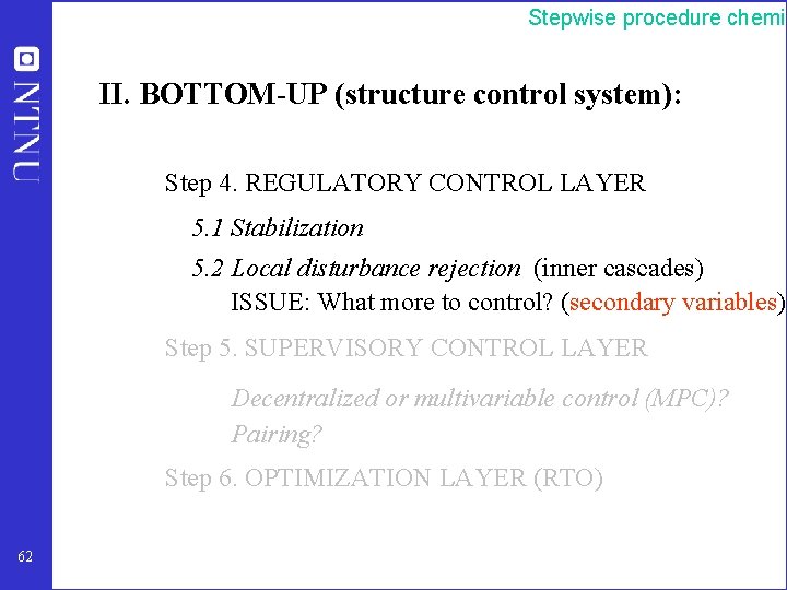
Stepwise procedure chemic II. BOTTOM-UP (structure control system): Step 4. REGULATORY CONTROL LAYER 5. 1 Stabilization 5. 2 Local disturbance rejection (inner cascades) ISSUE: What more to control? (secondary variables) Step 5. SUPERVISORY CONTROL LAYER Decentralized or multivariable control (MPC)? Pairing? Step 6. OPTIMIZATION LAYER (RTO) 62
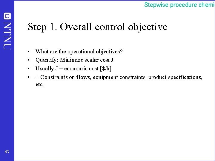
Stepwise procedure chemic Step 1. Overall control objective • • 63 What are the operational objectives? Quantify: Minimize scalar cost J Usually J = economic cost [$/h] + Constraints on flows, equipment constraints, product specifications, etc.
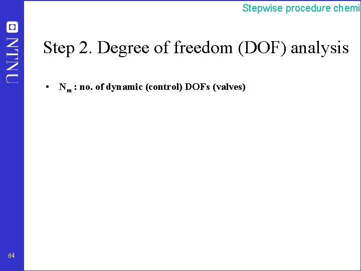
Stepwise procedure chemic Step 2. Degree of freedom (DOF) analysis • Nm : no. of dynamic (control) DOFs (valves) 64
Stepwise procedure chemic Step 3. What should we control? (primary controlled variables) • Intuition: “Dominant variables” • Systematic: Define cost J and minimize w. r. t. DOFs – Control active constraints (constant setpoint is optimal) – Remaining DOFs: Control variables c for which constant setpoints give small (economic) loss Loss = J - Jopt(d) when disturbances d occurs 65
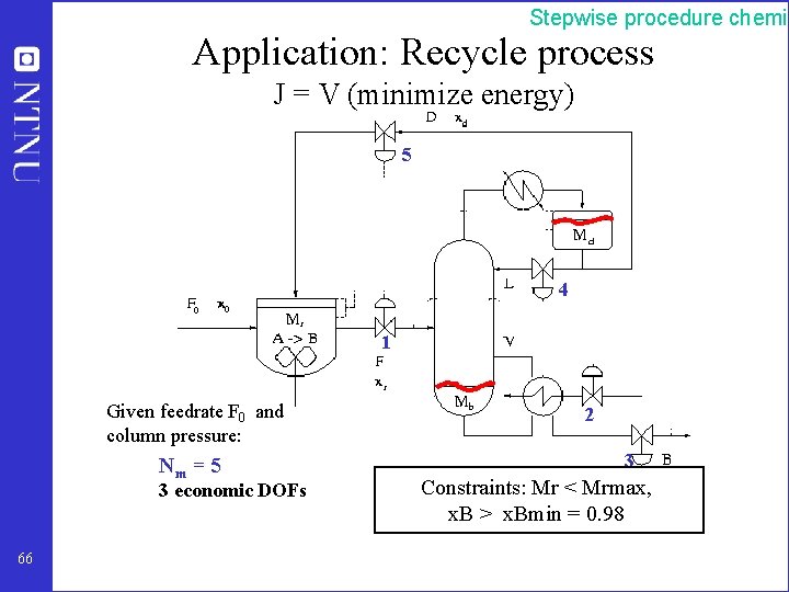
Stepwise procedure chemic Application: Recycle process J = V (minimize energy) 5 4 1 Given feedrate F 0 and column pressure: Nm = 5 3 economic DOFs 66 2 3 Constraints: Mr < Mrmax, x. B > x. Bmin = 0. 98
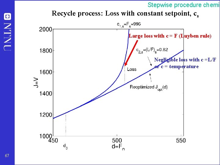
Stepwise procedure chemic Recycle process: Loss with constant setpoint, cs Large loss with c = F (Luyben rule) Negligible loss with c =L/F or c = temperature 67
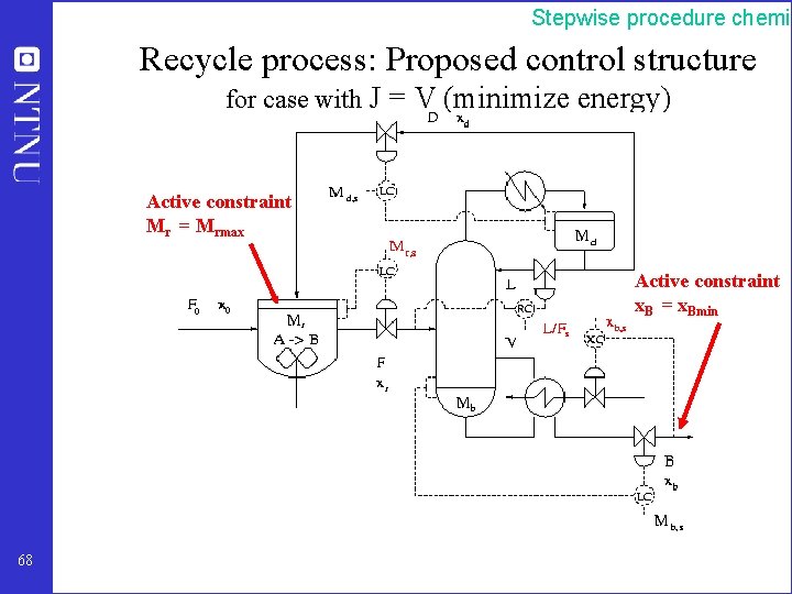
Stepwise procedure chemic Recycle process: Proposed control structure for case with J = V (minimize energy) Active constraint Mr = Mrmax Active constraint x. B = x. Bmin 68
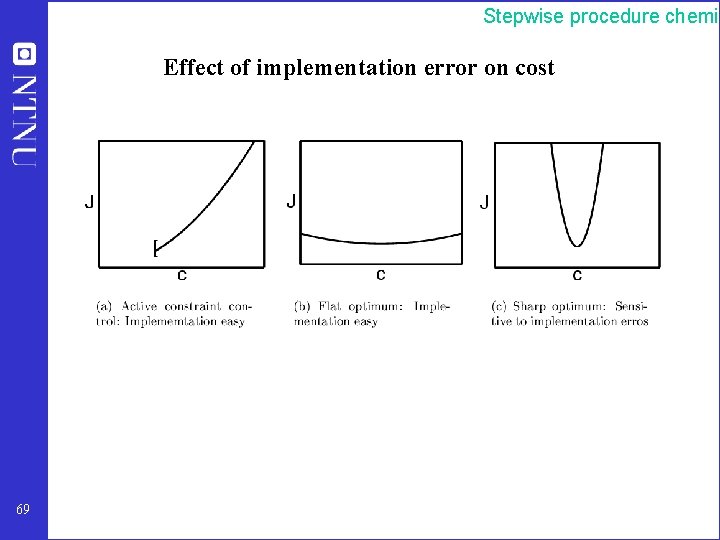
Stepwise procedure chemic Effect of implementation error on cost 69
Stepwise procedure chemic II. Bottom-up assignment of loops in control layer • Identify secondary (extra) controlled variable • Determine structure (configuration) of control system (pairing) • A good control configuration is insensitive to parameter changes! Industry: most common approach is to copy old designs 70
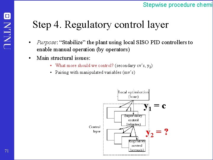
Stepwise procedure chemic Step 4. Regulatory control layer • Purpose: “Stabilize” the plant using local SISO PID controllers to enable manual operation (by operators) • Main structural issues: • What more should we control? (secondary cv’s, y 2) • Pairing with manipulated variables (mv’s) y 1 = c y 2 = ? 71
Stepwise procedure chemic Selection of secondary controlled variables (y 2) • The variable is easy to measure and control • For stabilization: Unstable mode is “quickly” detected in the measurement (Tool: pole vector analysis) • For local disturbance rejection: The variable is located “close” to an important disturbance (Tool: partial control analysis). 72
Stepwise procedure chemic Summary Procedure plantwide control: I. Top-down analysis to identify degrees of freedom and primary controlled variables (look for self-optimizing variables) II. Bottom-up analysis to determine secondary controlled variables and structure of control system (pairing). • Skogestad, S. (2000), “Plantwide control -towards a systematic procedure”, Proc. ESCAPE’ 12 Symposium, Haag, Netherlands, May 2002. • Larsson, T. and S. Skogestad, 2000, “Plantwide control: A review and a new design procedure”, Modeling, Identification and Control, 21, 209 -240. • Skogestad, S. (2000). “Plantwide control: The search for the self-optimizing control structure”. J. Proc. Control 10, 487507. 73 See also the home page of Sigurd Skogestad: http: //www. chembio. ntnu. no/users/skoge/
Biological systems • ”Self-optimizing” controlled variables have presumably been found by natural selection • Need to do ”reverse engineering” : – Find the controlled variables used in nature – From this identify what overall objective the biological system has been attempting to optimize 74
Conclusion • Negative Feedback is an extremely powerful tool • Complex systems can be controlled by hierarchies (cascades) of singleinput-single-output (SISO) control loops • Control extra local variables (secondary outputs) to avoid fundamental feedback control limitations • Control the right variables (primary outputs) to achieve ”selfoptimizing control” 75
- Slides: 75