Feature Squeezing Detecting Adversarial Examples in Deep Neural

Feature Squeezing: Detecting Adversarial Examples in Deep Neural Networks Weilin Xu David Evans Yanjun Qi

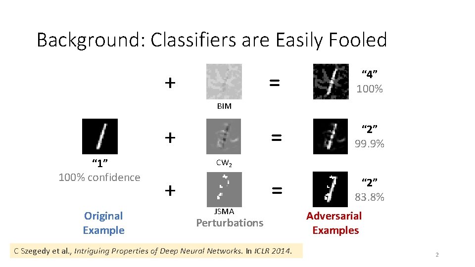
Background: Classifiers are Easily Fooled + = “ 4” 100% = “ 2” 99. 9% = “ 2” 83. 8% BIM + “ 1” 100% confidence Original Example CW 2 + JSMA Perturbations C Szegedy et al. , Intriguing Properties of Deep Neural Networks. In ICLR 2014. Adversarial Examples 2

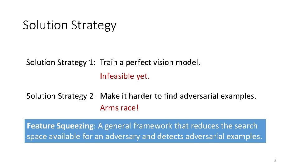
Solution Strategy 1: Train a perfect vision model. Infeasible yet. Solution Strategy 2: Make it harder to find adversarial examples. Arms race! Feature Squeezing: A general framework that reduces the search space available for an adversary and detects adversarial examples. 3

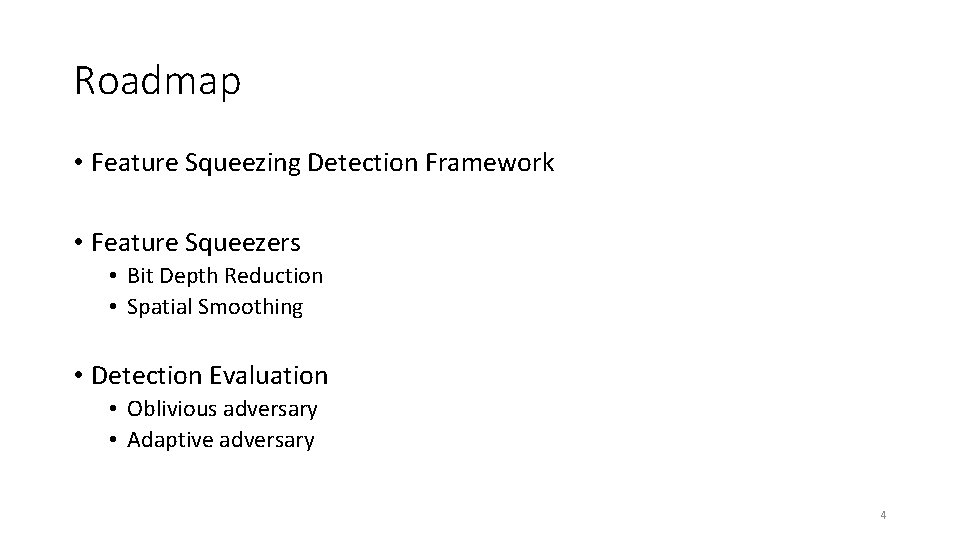
Roadmap • Feature Squeezing Detection Framework • Feature Squeezers • Bit Depth Reduction • Spatial Smoothing • Detection Evaluation • Oblivious adversary • Adaptive adversary 4

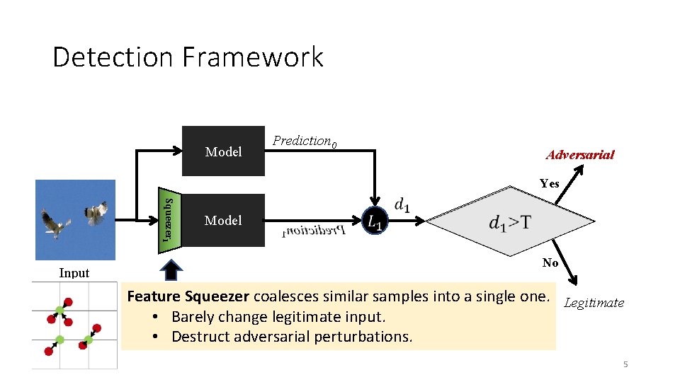
Detection Framework Model Prediction 0 Adversarial Yes Squeezer 1 Input Model No Feature Squeezer coalesces similar samples into a single one. Legitimate • Barely change legitimate input. • Destruct adversarial perturbations. 5

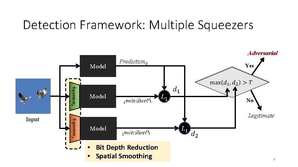
Detection Framework: Multiple Squeezers Adversarial Model Prediction 0 Yes Squeezer 1 Squeezer 2 Input Model No Legitimate Model • Bit Depth Reduction • Spatial Smoothing 6

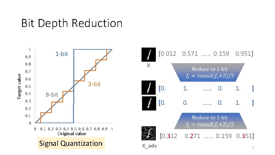
Bit Depth Reduction 1 0. 9 [0. 012 0. 571 …… 0. 159 0. 951] 1 -bit Target value 0. 8 X 0. 7 0. 6 3 -bit 0. 5 0. 4 0. 3 [0. 1. …… 0. 1. ] 8 -bit [0. …… 0. 1. ] 0. 2 0. 1 0 0 0. 1 0. 2 0. 3 0. 4 0. 5 0. 6 0. 7 0. 8 0. 9 1 Original value Signal Quantization [0. 312 0. 271 …… 0. 159 0. 351] X_adv 7

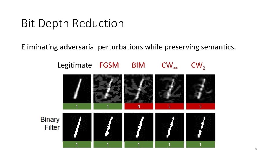
Bit Depth Reduction Eliminating adversarial perturbations while preserving semantics. Legitimate FGSM BIM CW∞ CW 2 1 1 4 2 2 1 1 1 8

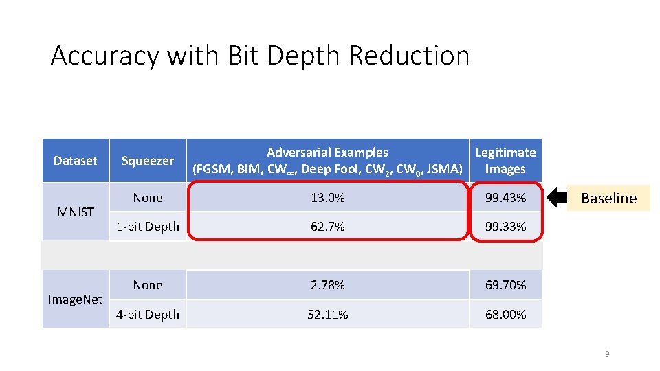
Accuracy with Bit Depth Reduction Dataset MNIST Image. Net Squeezer Adversarial Examples Legitimate (FGSM, BIM, CW∞, Deep Fool, CW 2, CW 0, JSMA) Images None 13. 0% 99. 43% 1 -bit Depth 62. 7% 99. 33% None 2. 78% 69. 70% 4 -bit Depth 52. 11% 68. 00% Baseline 9

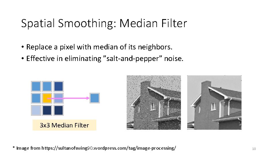
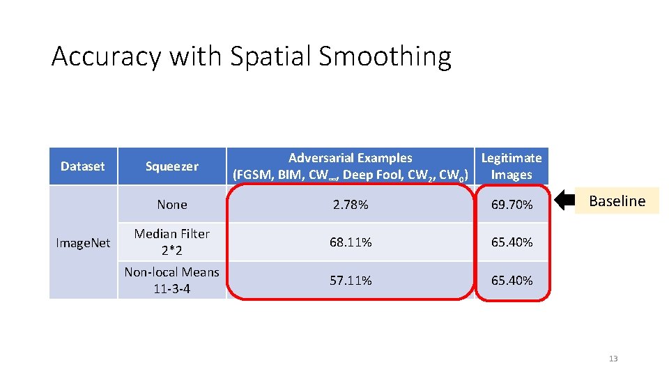
Spatial Smoothing: Median Filter • Replace a pixel with median of its neighbors. • Effective in eliminating ”salt-and-pepper” noise. 3 x 3 Median Filter * Image from https: //sultanofswing 90. wordpress. com/tag/image-processing/ 10

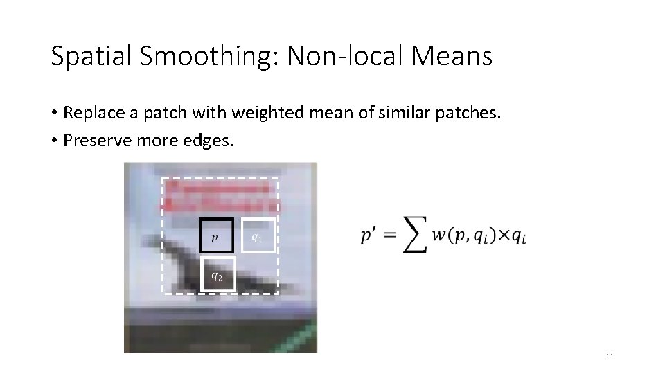
Spatial Smoothing: Non-local Means • Replace a patch with weighted mean of similar patches. • Preserve more edges. 11

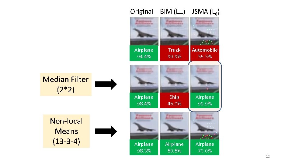
Original BIM (L∞) JSMA (L 0) Median Filter (2*2) Non-local Means (13 -3 -4) Airplane 94. 4% Truck 99. 9% Automobile 56. 5% Airplane 98. 4% Ship 46. 0% Airplane 99. 9% Airplane 98. 3% Airplane 80. 8% Airplane 70. 0% 12

Accuracy with Spatial Smoothing Dataset Image. Net Squeezer Adversarial Examples Legitimate (FGSM, BIM, CW∞, Deep Fool, CW 2, CW 0) Images None 2. 78% 69. 70% Median Filter 2*2 68. 11% 65. 40% Non-local Means 11 -3 -4 57. 11% 65. 40% Baseline 13

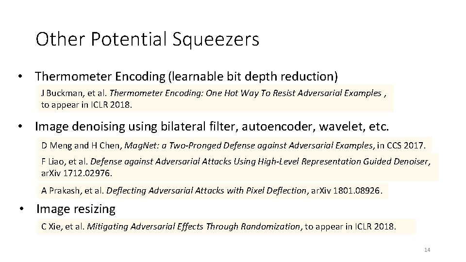
Other Potential Squeezers • Thermometer Encoding (learnable bit depth reduction) J Buckman, et al. Thermometer Encoding: One Hot Way To Resist Adversarial Examples , to appear in ICLR 2018. • Image denoising using bilateral filter, autoencoder, wavelet, etc. D Meng and H Chen, Mag. Net: a Two-Pronged Defense against Adversarial Examples, in CCS 2017. F Liao, et al. Defense against Adversarial Attacks Using High-Level Representation Guided Denoiser, ar. Xiv 1712. 02976. A Prakash, et al. Deflecting Adversarial Attacks with Pixel Deflection, ar. Xiv 1801. 08926. • Image resizing C Xie, et al. Mitigating Adversarial Effects Through Randomization, to appear in ICLR 2018. 14

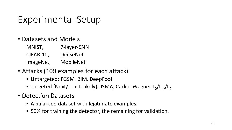
Experimental Setup • Datasets and Models MNIST, 7 -layer-CNN CIFAR-10, Dense. Net Image. Net, Mobile. Net • Attacks (100 examples for each attack) • Untargeted: FGSM, BIM, Deep. Fool • Targeted (Next/Least-Likely): JSMA, Carlini-Wagner L 2/L∞/L 0 • Detection Datasets • A balanced dataset with legitimate examples. • 50% for training the detector, the remaining for validation. 15

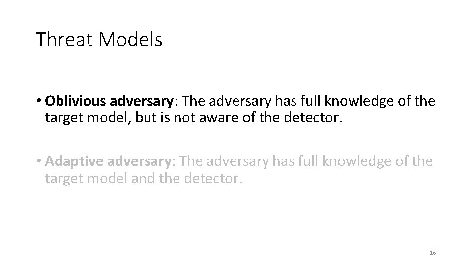
Threat Models • Oblivious adversary: The adversary has full knowledge of the target model, but is not aware of the detector. • Adaptive adversary: The adversary has full knowledge of the target model and the detector. 16

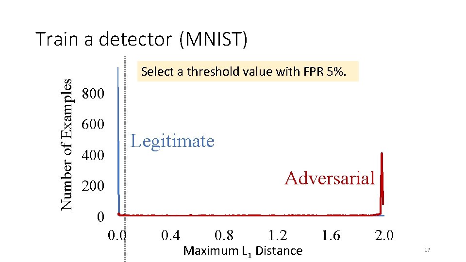
Number of Examples Train a detector (MNIST) Select a threshold value with FPR 5%. 800 600 Legitimate 400 Adversarial 200 0 0. 4 0. 8 1. 2 Maximum L 1 Distance 1. 6 2. 0 17

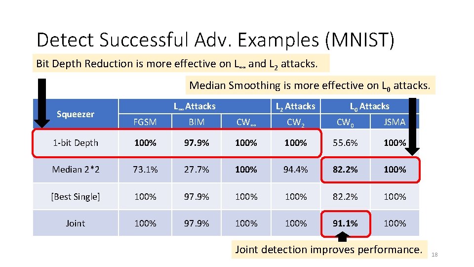
Detect Successful Adv. Examples (MNIST) Bit Depth Reduction is more effective on L∞ and L 2 attacks. Median Smoothing is more effective on L 0 attacks. Squeezer L∞ Attacks L 2 Attacks L 0 Attacks FGSM BIM CW∞ CW 2 CW 0 JSMA 1 -bit Depth 100% 97. 9% 100% 55. 6% 100% Median 2*2 73. 1% 27. 7% 100% 94. 4% 82. 2% 100% [Best Single] 100% 97. 9% 100% 82. 2% 100% Joint 100% 97. 9% 100% 91. 1% 100% Joint detection improves performance. 18

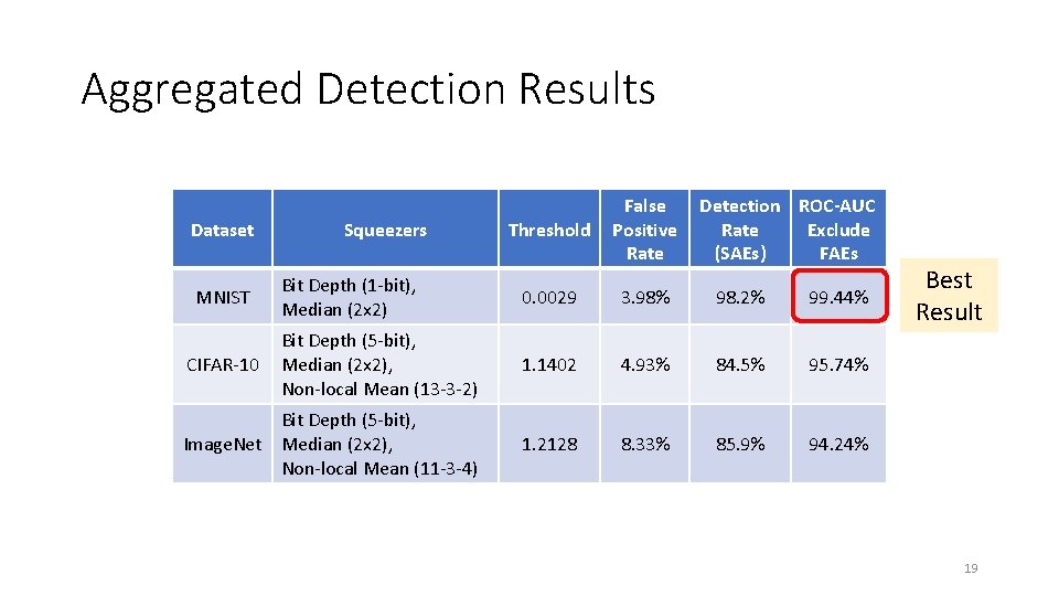
Aggregated Detection Results Threshold False Positive Rate Bit Depth (1 -bit), Median (2 x 2) 0. 0029 3. 98% 98. 2% 99. 44% Bit Depth (5 -bit), Median (2 x 2), Non-local Mean (13 -3 -2) 1. 1402 4. 93% 84. 5% 95. 74% Bit Depth (5 -bit), Image. Net Median (2 x 2), Non-local Mean (11 -3 -4) 1. 2128 8. 33% 85. 9% 94. 24% Dataset MNIST CIFAR-10 Squeezers Detection ROC-AUC Rate Exclude (SAEs) FAEs Best Result 19

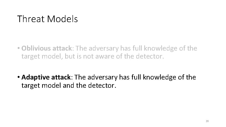
Threat Models • Oblivious attack: The adversary has full knowledge of the target model, but is not aware of the detector. • Adaptive attack: The adversary has full knowledge of the target model and the detector. 20

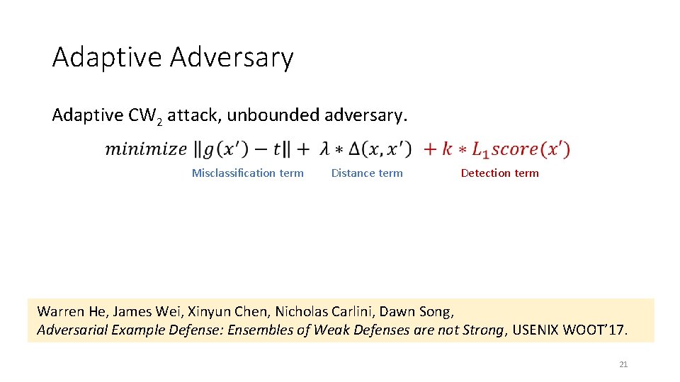
Adaptive Adversary Adaptive CW 2 attack, unbounded adversary. Misclassification term Distance term Detection term Warren He, James Wei, Xinyun Chen, Nicholas Carlini, Dawn Song, Adversarial Example Defense: Ensembles of Weak Defenses are not Strong, USENIX WOOT’ 17. 21

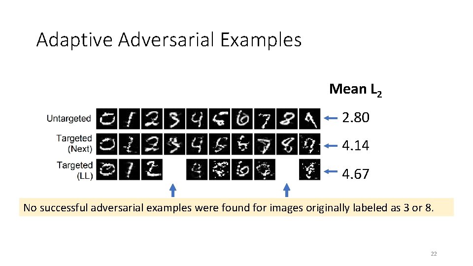
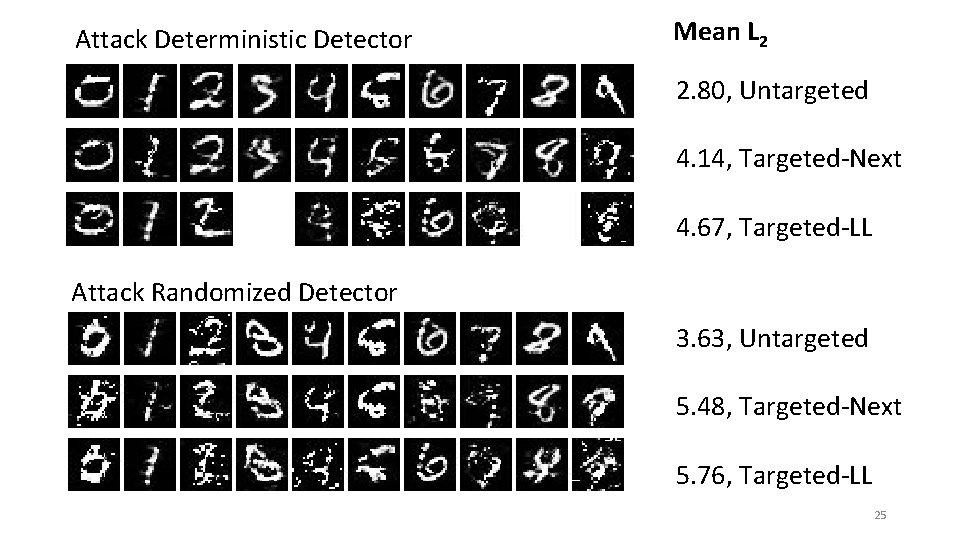
Adaptive Adversarial Examples Mean L 2 2. 80 4. 14 4. 67 No successful adversarial examples were found for images originally labeled as 3 or 8. 22

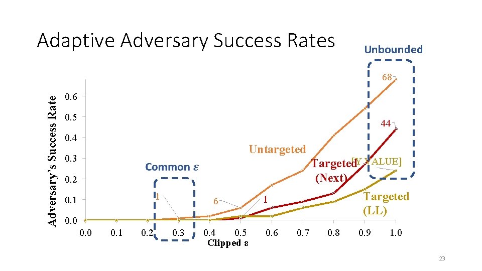
Adaptive Adversary Success Rates Unbounded Adversary’s Success Rate 68 0. 6 0. 5 44 0. 4 Untargeted 0. 3 0. 2 1 0. 1 6 [Y VALUE] Targeted (Next) Targeted (LL) 1 0. 0 0. 1 0. 2 0. 3 0. 4 0. 5 Clipped ε 0. 6 0. 7 0. 8 0. 9 1. 0 23

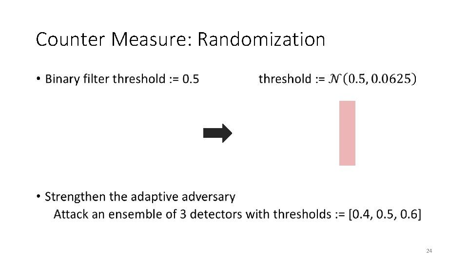
Counter Measure: Randomization • 24

Attack Deterministic Detector Mean L 2 2. 80, Untargeted 4. 14, Targeted-Next 4. 67, Targeted-LL Attack Randomized Detector 3. 63, Untargeted 5. 48, Targeted-Next 5. 76, Targeted-LL 25

Conclusion • Feature Squeezing hardens deep learning models. • Feature Squeezing gives advantages to the defense side in the arms race with adaptive adversary. 26

Thank you! Reproduce our results using Evade. ML-Zoo: https: //evade. ML. org/zoo 27

28

Backup Slides 29

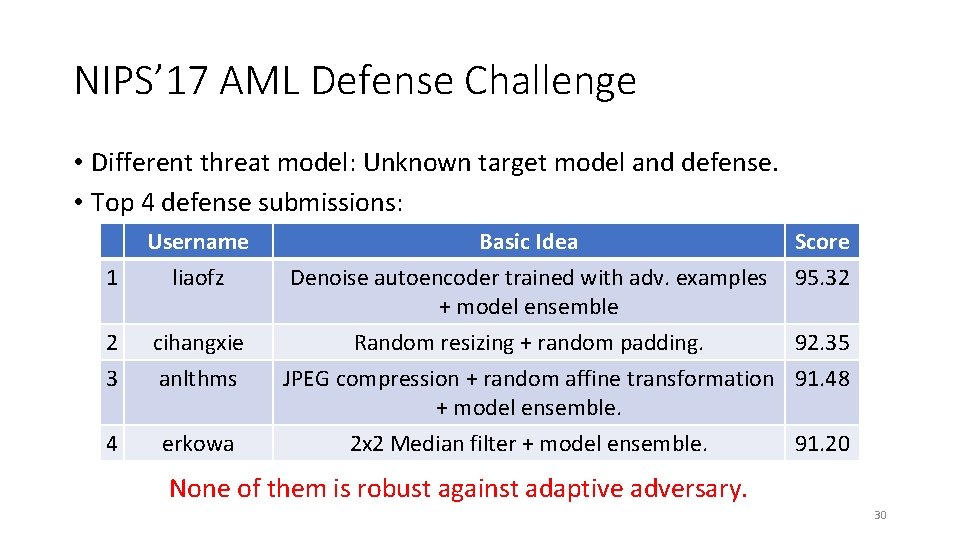
NIPS’ 17 AML Defense Challenge • Different threat model: Unknown target model and defense. • Top 4 defense submissions: Username 1 liaofz 2 cihangxie 3 anlthms 4 erkowa Basic Idea Score Denoise autoencoder trained with adv. examples 95. 32 + model ensemble Random resizing + random padding. 92. 35 JPEG compression + random affine transformation 91. 48 + model ensemble. 2 x 2 Median filter + model ensemble. 91. 20 None of them is robust against adaptive adversary. 30