Fault Modeling Simulation and Diagnosis Fault Modeling Faults

Fault Modeling, Simulation and Diagnosis

Fault Modeling Faults are the manifestations of physical defects. Logical fault modeling lead to a number of benefits. Reducing complexity Technology-independent modeling Achieving abstraction Logical faults Explicit – may be enumerated Implicit – can not be enumerated Structural – modify the interconnections among

Modeling levels Modeling can be done at different levels Geometrical to functional levels

Combinational circuits Consider an n input fault free combinational circuit C whose output is F. Presence of fault f transforms C into differenct circuit Cf with output Ff(x) Let t represents specific input vector called test vector. F(t) response of C Test vector t is said to detect fault f iff F(t)!=Ff(t)

Sequential circuit Circuit SC Has initial state q Output F Fault f and output Scf Need for a sequence of tests

Sensitized path In a given circuit , a line whose value under test t changes in the presence of fault f is said to be sensitized to the fault f by test t. A path composed of sensitized lines is called a sensitized path. The test t propagates the fault effect along a sensitized path.

Example Fault x/1 is sensitized by the value 0 on line x. Test t=1011 is simulated without fault and with fault. Observe output in the two cases.

Structural fault models Stuck-at fault model Bridging fault model The Single Stuck-Fault model (SSF)

Structural fault models Stuck-at fault model In this case, a line l is assumed to be stuck at a fixed logic value v, v E {0, 1} Two stuck at faults exists: a line l is stuck-at-1 (l/1 or l s-a-1) Or line l stuck-at-0 (l/0 or l s-a-0) A short between ground (s-a-0) or power (s-a-1)

Structural fault models Bridging fault model This represents the case of shorts between signal lines. The short between two lines can be modeled as the ANDing (Oring) of the functions realized by the lines depending on the technology used.

Structural fault models The Single Stuck-Fault model (SSF) Is the standard or traditional fault model Extensively used at modeling single stuck-at faults in digital circuits. If the number of possible SSF sites is n, then there are 2 n possible SSFs. Each site can be s-a-0 or s-a-1. The number of sites in which SSF may occur can be computed: n=sum( 1+fi-qi) from 1 to m Where qi= 1 if fi=1 , qi = 0 if fi>1 m=signal sources and fi=fan out count of signal

SSF It can be used to model a number of different physical faults It is technology independent Tests that detect SSF s detect a number of other non-classical faults

Detectable fault A fault f is said to be detectable if there exists at least one test t that detects f, otherwise , f is an undetectable fault. The presence of an undetectable fault f may prevent the detection of another fault g, even then when there exists a test which detects the fault g.

Example Fault b/1 is undetectable Test t = 1101 detects fault a/0 In the presence of b/1 test t can not detect the fault a/0

Example The test T = {1111, 0111, 1110, 1001, 1010, 0101} detects every SSF in the circuit show in the diagram. Let f be b/1 and g be c/1 The only test in T that detects the single faults f and g is 1001. Multiple fault {f, g} can not be detected under the test vector 1001, f masks g and g masks f.

Multiple faults Let T be the set of all tests that detects a fault f. A fault g functionally masks fault f iff the multiple fault {g & f} is not detected by any test t E T. Equivalent faults: two faults fi and fj are said to be equivalent if every test that detects fi also detects fj and vice versa. i. e. tests for fi and fj are identical.

Multiple faults The s_a_0 faults on the input and output of a 2 -input AND gate are equivalent. Fault dominance: Let Tf be the set of all tests that detects a fault f. We say that a fault g dominates fault f iff g and f are functionally equivalent under Tf. If fault g dominates fault f then the test t that detects f will also detect g. Fault dominance is important as by deriving a test to detect f we automatically obtain a test that detects g as well. One criterion for choosing a fault model is that of having its faults dominated by a number of other faults.

Multiple faults single_stuck_at model SSF possesses such property. Fault collapsing refers to the reduction of the set of faults need to be analyzed.

Fault Collapsing Two types of fault collapsing: 1. Equivalence fault collapsing 2. Dominance fault collapsing

Fault Collapsing- Equivalence fault collapsing Refers to the reduction in the set of faults based on equivalence relations. e. g. a gate with a controlling input value c and inversion i, all input s-a-c faults and the output sa-(c. XORi) are functionally equivalent.

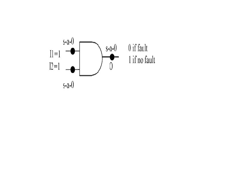
Fault Equivalence For Single Stuck. At Fault Model Two stuck-at faults f 1 and f 2 are called equivalent iff the output function represented by the circuit with f 1 is same as the output function represented by the circuit with f 2. Equivalent faults have exactly the same set of test patterns. In the AND gate of Figure 1, all stuck-at-0 faults are equivalent as they transform the circuit to O=0 and have I 1=1, I 2=1 as the test pattern.

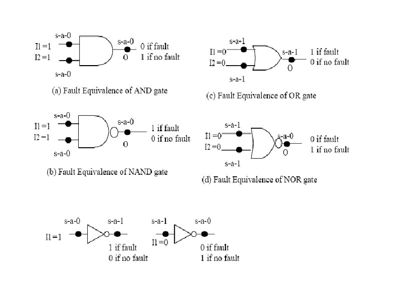
Single Stuck-At Fault Model Now lets us see what stuck-at faults are equivalent in other logic gates. Figure 2 illustrates equivalent faults in AND, NAND , OR , NOR gates and Inverter with the corresponding test patterns.

2. Dominance fault collapsing Refers to the reduction in the set of faults based on dominance relations. In general for a gate with controlling input value c and inversion i, the output fault s-a-(c^ XOR i) dominates any input s-a-c^ fault. If all tests of a stuck-at fault f 1 detect fault f 2 then f 2 dominates f 1. If f 2 dominants f 1 then f 2 can be removed and only f 1 is retained.

Redundant faults A combinational circuit that contains an undetectable stuck-at fault is said to be redundant. Such circuit can always be simplified by removing some gate(s) or gate input(s). Example: an input OR gate with a constant 0 value on one input is logically equivalent to (n-1) input OR gate input s-a-1 is undetectable, the OR gate can be removed and replaced by constant 1 signal.

Reduction rules Undetectable fault Reduction rule OR(NOR) input s-a-0 Remove input OR(NOR) input s-a-1 Remove gate and replace by 1 (0) AND(NAND) input s-a-1 Remove input AND(NAND) input s-a-0 Remove gate, replace by 0(1)

Fault simulation is the process of determining the fault coverage, either as fraction or as a percentage of the modeled faults detected by a given set of inputs (test vectors) as well as finding the set of undetected faults in the modeled circuit. Input to fault simulator: circuit, a specified sequence of test vectors, fault model.

Fault simulator The output of fault simulator is measured using a number of parameters. 1. set of undetected faults The smaller the undetected faults the better the simulator. 2. fault coverage= detected faults/ simulated faults * 100

Fault simulation algorithms Serial fault simulation algorithm Parallel fault simulation Deductive fault simulation Concurrent fault simulation Critical path tracing

Serial fault simulation algorithm True-value simulation is performed across all vectors and outputs saved. Faulty circuits are simulated one-by-one by modifying the circuit and running true value simulator. Simulation of a faulty circuit stops as soon as fault is detected.

Serial algorithm a) simulate fault free circuit and save responses b) repeat the following steps for each fault on the fault list b. 1. Modify the net-list by injecting one fault b. 2 simulate modified net-list(one vector at a time) b. 3 Compare obtained response with saved response. b. 4 In the case of discrepancy, declare fault as detected and stop simulation ; otherwise fault is declared as undetected.

Parallel fault simulation Takes advantage of available bit-parallelism in logical operations of a digital computer in processing computer words. 64 -bit word computer it is possible to simulate upto 64 different copies of the simulated circuit, each bit can represent the status of a circuit such that if the circuit is fault free, then the corresponding bit is 1; otherwise the bit will be 0.

Parallel fault simulation If the computer word size is N, then N-1 copies of faulty circuit are also generated. For a total of M faults in the circuit M/N-1 simulation runs will be needed. Spped up of (N-1) over serial simulator. Example

Deductive fault simulation Only the fault free circuit is simulated. Faulty circuits are deduced from the fault free one. The simulator processes all faults in a single pass using true-value simulation. Makes the simulator fast. A vector is simulated in true-value mode.

Deductive fault simulation A deductive procedure is performed on all lines in level-order from inputs to outputs. LA= fault list- the set containing the name of every fault that produces an error on line A when the circuit is in its current logic state. Fault lists are to be propagated from the primary inputs (PIs) to primary outputs (Pos). A fault list is generated for each signal lines, and updated as necessary with every change in the logic state of the circuit.

Deductive fault simulation List events occur when a fault list changes. Instead of keeping all signal values, as in the parallel fault simulation, only those bits that are different from the good values are kept in deductive fault simulation.

Example

Concurrent fault simulation This technique extends the event driven simulation of faults. The fault is only simulated when it causes some lines to carry a different value than the corresponding one in the fault free-circuit. A fault list is associated with each element. An entry in the list contains the fault and the inputoutput value of the gate induced by the fault.

Example Circuit diagram and table

Critical path tracing A line l with value 0(1) is said to be critical under test pattern t iff t detects the fault line l s-a-1(0). 0(1) is called the critical value of that line. By finding the critical lines under a test t, it is possible to know the faults detected by t. Example: if a line l has value 1 and is critical under test t, then the fault line l s-a-0 can be detected by t. Fault simulation by critical path tracing determines those critical lines by a back-tracking process starting from the primary outputs and

Example Critical path simulation example

Fault Diagnosis Combinational fault diagnosis Sequential fault diagnosis methods

Fault Diagnosis (FD) is defined as the process of locating fault(s) in a given circuit. Two main fault diagnosis processes are: Top down process Bottom up process

Fault Diagnosis Top down process: Large units such as Printed Circuit Boards (PCBs) are first diagnosed. Faulty PCBs are then tested in a repair center to locate the faulty ICs. Used while the system is in operation.

Fault Diagnosis Bottom up process: Components are first tested and only fault free ones are used to assemble higher level systems. Used at the time of manufacturing

Combinational fault diagnosis According to this approach, the fault simulation is used to determine the possible responses to a given test in the presence of faults. This step helps constructing fault table (FT) or fault dictionary (FD). To locate fault, a match, using a table look-up, between the actual results of test experiments and one of the precomputed (expected) results stored in FT is sought.

Combinational fault diagnosis A fault table is a matrix FT = ||aij|| where columns Fj represents faults, rows Ti represents test patterns. Aij=1 if the test pattern ti detects fault Fj otherwise aij=0. If this look-up is successful, the FT (FD) provides the corresponding faults. The actual result of a given test pattern is indicated as a 1 if it differs from the precomputed expected one, otherwise it is 0. The result of a test experiment is represented by

Three cases Total match: the test result E matches with a single column vector fi in FT. This result corresponds to the case where a single fault Fj has been located. Maximum diagnostic resolution has been obtained. Diagnostic resolution (DR) is used to define the degree of accuracy to which faults can be located in the circuit under test (CUT).

Three cases Partial match: the test result E matches with a subset of column vectors {fi, fj, . . . , fk} in FT. This result corresponds to the case where a subset of indistinguishable faults {Fi, Fj, . . . , Fk} has been located. Faults that can not be distinguishable are called Functionally equivalent faults (FEFs).

Three cases No match: the test result E does not match with any column vectors in FT. This result corresponds to the case where the given set of vectors does not allow to carry out fault diagnosis. The set of faults described in the fault table must be incomplete.

Example Table

Sequential fault diagnosis methods In sequential fault diagnosis the process of fault location is carried out step by step. Each step depends on the result of the diagnostic experiment at the previous step. Sequential experiments can be carried out either by observing only output responses of the CUT or by pinpointing by a special probe. Procedure can be graphically represented as diagnostic tree.

Sequential fault diagnosis methods Diagnostic tree- consists of fault nodes (FN) and test nodes (TN) FN is labeled by a set of not yet distinguished faults. The starting fault is labeled by the set of all faults. To each Fnk a TN is linked labeled by a test pattern tk to be applied next. Every test pattern distinguishes between the faults it detects and the ones it does not. The test pattern tk divides the faults in FNk into

Sequential fault diagnosis methods Each test node has two outgoing edges corresponding to the results of the experiment of this test pattern. The results are indicated as pass (P) or failed (F).

Example diagnostic tree diagram

Example Circuit diagram F 1: c 1 s-a-0 F 2: d s-a-1

Guided probe testing Extends the testing process by monitoring internal signals in the CUT via a probe which is moved following the guidance provided by the test equipment. The principle of guided probe testing is to back trace an error from the primary output where it has been observed during edge pin testing to its physical location in the CUT. Probing is carried out step by step. In each step an internal signal is probed and compared to the expected value.