Fast Pattern Matching in Non Linear ToneMapped Images

Fast Pattern Matching in Non. Linear Tone-Mapped Images Yacov Hel-Or The Interdisciplinary Center (IDC), Israel Visiting Scholar - Google Hagit Hel-Or and Eyal David U. of Haifa, Israel 1

Pattern Matching under Tone Mapping • A given pattern p is sought in an image. • The pattern may appear at any location in the image. • The image may be subject to some tone changes. pattern image similarity 2

Pattern Matching • Source of Tone Changes: – Illumination conditions – Camera parameters – Different Modalities • Applications: “patch based” methods – Image summarization – Image retargeting – Image editing – Super resolution – Tracking, Recognition, many more …

Tone Changes as Tone Mappings • Assumption: Tone changes can be locally represented as a Tone Mapping between the sought pattern p and a candidate window w: Vw w=M(p) Vp or p=M(w) Vp 4

Distance Metric • Given a pattern p and a candidate window w a distance metric must be defined, according to which matchings are determined: D (p , w ) • Desired properties of D(p, w) : – Discriminative – Robust to Noise – Invariant to some deformations: tone mapping – Fast to execute

Most Common Distance Metrics • Sum of Squared Difference (SSD): – By far the most common solution. – Assumes the identity tone mapping. – Fast implementation (~1 convolution).

• Normalized Cross Correlation (NCC): – Compensates for linear mappings. – Fast implementation (~ 1 convolution).

• Mutual Information (MI): D(p, w)=I(p, w)=H(w)-H(w | p) – Measures the statistical dependencies between p and w. – Compensates for non-linear mappings. H(p) H(w)

MI as a Distance Measure: Properties: • Measures the entropy loss in w given p. • Highly Discriminative. • Sensitive to bin-size / kernel-variance. • Inaccurate for small patched. • Very slow to apply. I(w, p) H(w) H(p)

Proposed Approach: Matching by Tone Mapping (MTM) Properties: • Highly discriminative. • Invariant to any (non-linear) tone mapping. • Robust to noise. • Very fast to apply. • Natural generalization of the NCC for non-linear mappings.

Matching by Tone Mapping (MTM) • Proposed distance measure: • Note: the division by var(w) avoids the trivial mapping.

How can MTM be calculated efficiently? Basic Ideas: • Approximate M(p) by a piece-wise constant mapping. Vw Vw Vp • Enables to represent M(p) in a linear form. • The minimization can be solved in closed form. Vp

Tone Mapping as a linear form: • Assume the pattern/window values are restricted to the half open interval [a, b). • We divide [a, b) into k bins =[ 1, 2, . . . , k+1] 1 j+1 j 2 k+1 z • A value z is naturally associated with a single bin: B(z)=j if z [ j, j+1)

Pattern Slices • We define a pattern slice

Pattern Slices 0 1 • We define a pattern slice 2 nd slice p 2 1 st slice p 1

The Slice Matrix = Sp • Raster scanning the slice windows and stacking into a matrix constructs a slice matrix Sp =[p 1 p 2 … pk].

Sp * p • The matrix Sp is orthogonal: pi pj = |pi| ij • Its columns span the space of piecewise constant tone mappings of p: Sp p

Sp * p M(p) Changing the values to a different vector, , applies piecewise tone mapping: S p M(p)

Back to Pattern Matching • Representing tone mapping in a linear form, D(p, w) boils down to: • The above minimization can be solved in closed form:

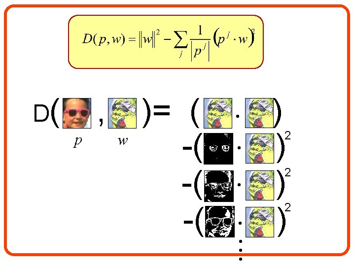
MTM for running windows: 2 ( ( * box filter ) 2 * ) Pattern

MTM for running windows: p 2 : ( 2 * ) Pattern

Complexity • Convolutions can be applied efficiently since pj is sparse. • Convolving with pj requires |pj| operations. • Since pi pj= run time for all k sparse convolutions sum up to a single convolution!

MTM and Other Distances • The MTM can be shown to measure: • This is related to the Correlation-Ratio distance measure (Pearson 1930, Roche et al. 1998) and the Fisher’s LD. • Restricting M to be a linear tone mapping: M(z)=az+b, the MTM distance D(w, p) reduces to the NCC.

MTM and MI • MTM and MI are similar in spirit: • While MI maximizes the entropy reduction in (w | p) MTM maximizes the variance reduction in (w | p). • However, MTM outperforms MI with respect to speed and accuracy (in small patch cases).

Results

Detection rates (over 2000 image pattern pairs) v. s extremity of the applied tone mapping. 28

Run time for various pattern sizes (in 512 x 512 image) 29

Performance of MI and MTM for various pattern sizes and over various bin-sizes 30

Example Application: Shadow Detection in Video • How can we distinguish between target and background? Background model Current video frame

Naïve Background Subtraction

• Assumption: Shadow patches are functionally dependent on the background patches. Background model Video frame

MTM distance

MTM distance

Conclusions: • A new distance measure that accounts for nonlinear tone mappings. • A very efficient scheme which can be applied over the entire image using ~1 convolution. • A natural generalization of NCC. 36

37