Fast Multipole Methods and the Fast Gauss Transform

Fast Multipole Methods and the Fast Gauss Transform Ramani Duraiswami Department of Computer Science and Institute for Advanced Computer Studies University of Maryland, College Park http: //www. umiacs. umd. edu/~ramani Joint work with Changjiang Yang, Nail A. Gumerov and Larry S. Davis NIPS: Fast N-body learning 12/17/2004

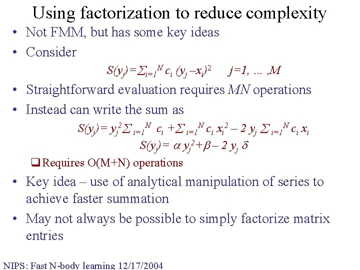
Using factorization to reduce complexity • Not FMM, but has some key ideas • Consider S(yj)= i=1 N ci (yj –xi)2 j=1, … , M • Straightforward evaluation requires MN operations • Instead can write the sum as S(yj)= yj 2 i=1 N ci + i=1 N ci xi 2 – 2 yj i=1 N ci xi S(yj)= yj 2+ – 2 yj q. Requires O(M+N) operations • Key idea – use of analytical manipulation of series to achieve faster summation • May not always be possible to simply factorize matrix entries NIPS: Fast N-body learning 12/17/2004

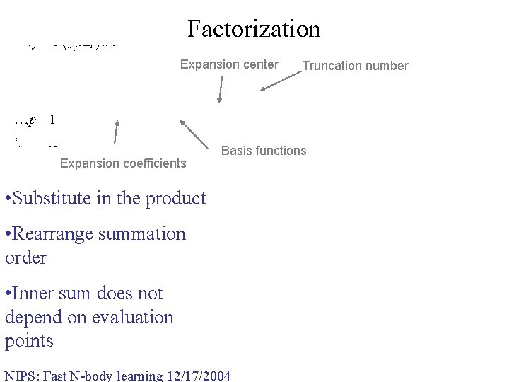
Factorization Expansion center Expansion coefficients Truncation number Basis functions • Substitute in the product • Rearrange summation order • Inner sum does not depend on evaluation points NIPS: Fast N-body learning 12/17/2004

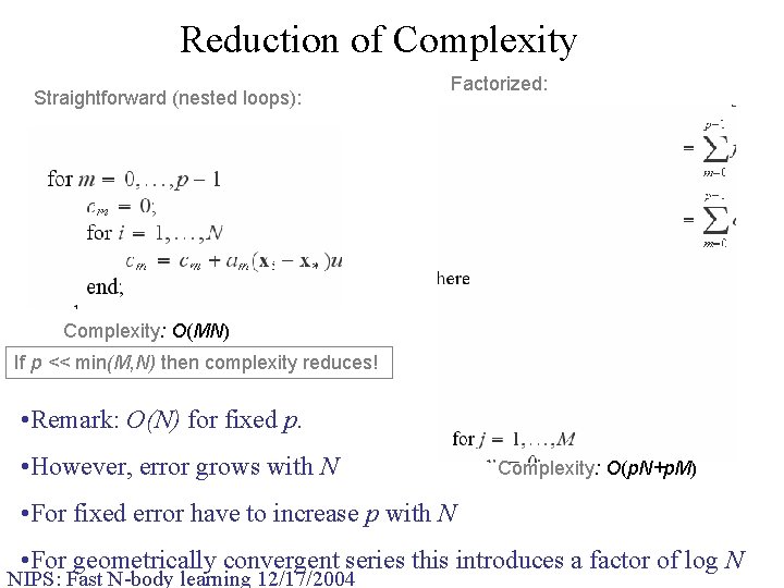
Reduction of Complexity Straightforward (nested loops): Factorized: Complexity: O(MN) If p << min(M, N) then complexity reduces! • Remark: O(N) for fixed p. • However, error grows with N Complexity: O(p. N+p. M) • For fixed error have to increase p with N • For geometrically convergent series this introduces a factor of log N NIPS: Fast N-body learning 12/17/2004

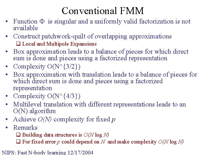
Conventional FMM • Function is singular and a uniformly valid factorization is not available • Construct patchwork-quilt of overlapping approximations q Local and Multipole Expansions • Box approximation leads to a balance of pieces for which direct sum is done and pieces using a factorized representation • Complexity O(N^{3/2}) • Box approximation with translation leads to a balance of pieces for which direct sum is done and pieces using a factorized representation • Complexity O(N^{4/3}) • Multilevel translation with different representations leads to an O(N) algorithm • Achieve O(N) complexity for fixed p • Remarks q Building data structures is O(N log N) q For fixed error p could depend on N and make complexity O(N log N) NIPS: Fast N-body learning 12/17/2004

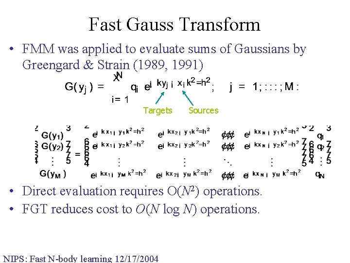
Fast Gauss Transform • FMM was applied to evaluate sums of Gaussians by Greengard & Strain (1989, 1991) Targets Sources • Direct evaluation requires O(N 2) operations. • FGT reduces cost to O(N log N) operations. NIPS: Fast N-body learning 12/17/2004

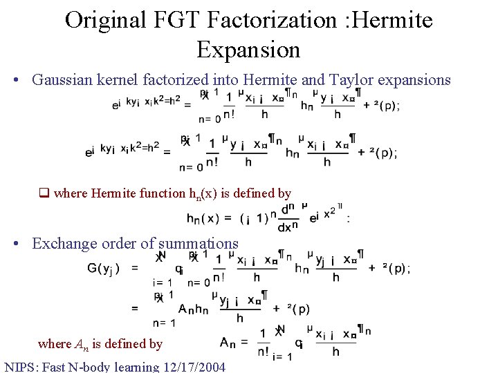
Original FGT Factorization : Hermite Expansion • Gaussian kernel factorized into Hermite and Taylor expansions q where Hermite function hn(x) is defined by • Exchange order of summations where An is defined by NIPS: Fast N-body learning 12/17/2004

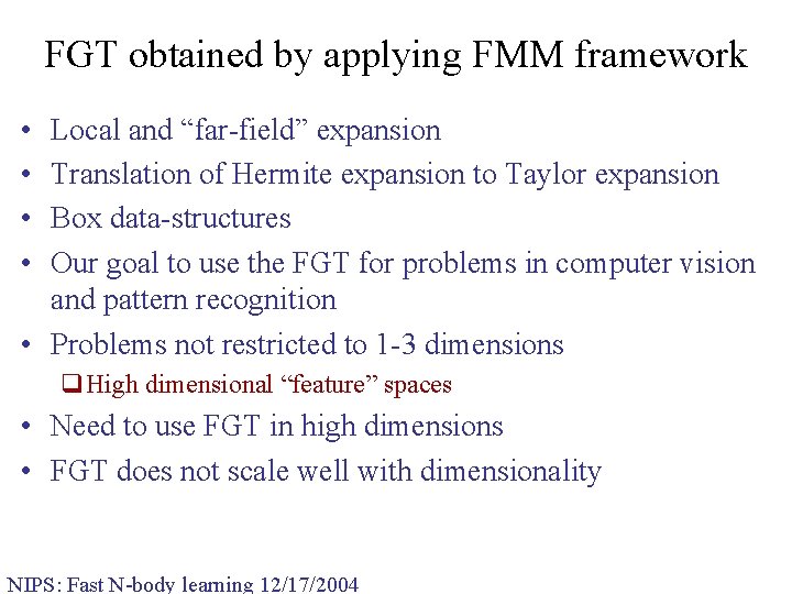
FGT obtained by applying FMM framework • • Local and “far-field” expansion Translation of Hermite expansion to Taylor expansion Box data-structures Our goal to use the FGT for problems in computer vision and pattern recognition • Problems not restricted to 1 -3 dimensions q. High dimensional “feature” spaces • Need to use FGT in high dimensions • FGT does not scale well with dimensionality NIPS: Fast N-body learning 12/17/2004

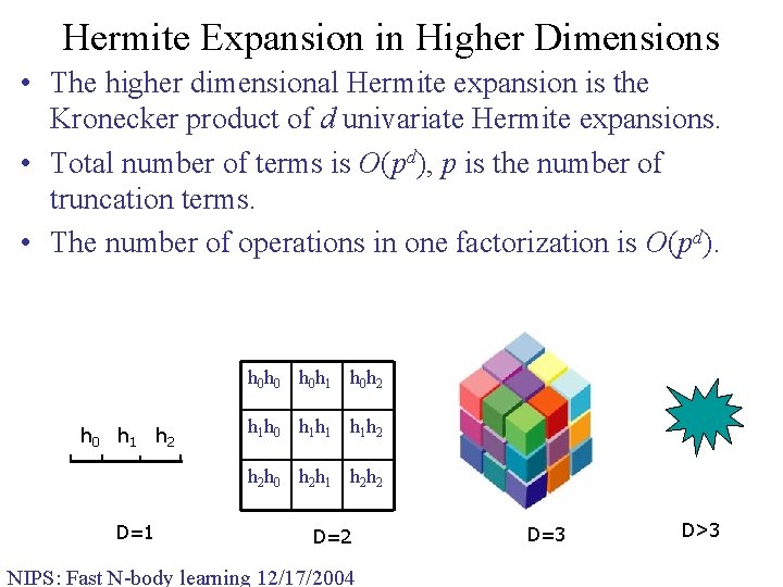
Hermite Expansion in Higher Dimensions • The higher dimensional Hermite expansion is the Kronecker product of d univariate Hermite expansions. • Total number of terms is O(pd), p is the number of truncation terms. • The number of operations in one factorization is O(pd). h 0 h 0 h 0 h 1 h 0 h 2 h 0 h 1 h 2 h 1 h 0 h 1 h 1 h 1 h 2 h 2 h 0 h 2 h 1 h 2 h 2 D=1 D=2 NIPS: Fast N-body learning 12/17/2004 D=3 D>3

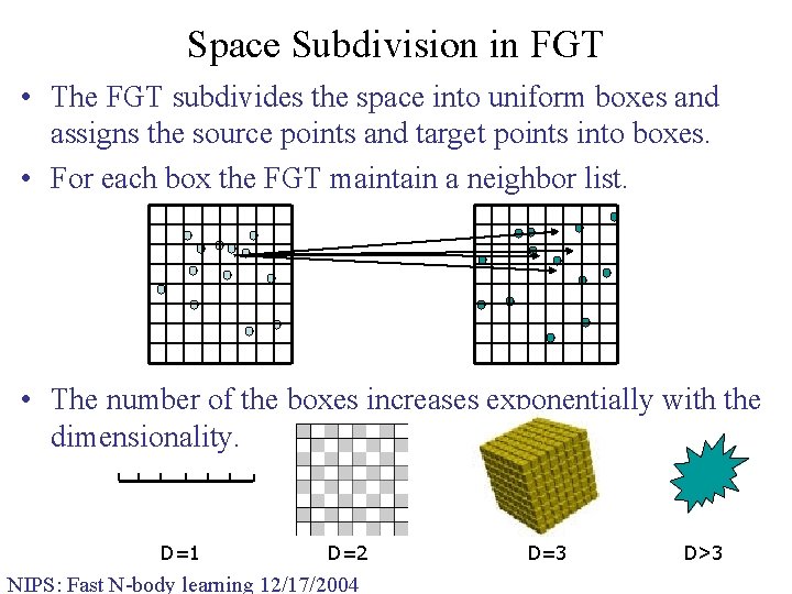
Space Subdivision in FGT • The FGT subdivides the space into uniform boxes and assigns the source points and target points into boxes. • For each box the FGT maintain a neighbor list. • The number of the boxes increases exponentially with the dimensionality. D=1 D=2 NIPS: Fast N-body learning 12/17/2004 D=3 D>3

FGT in Higher Dimensions • The higher dimensional Hermite expansion is the product of univariate Hermite expansion along each dimension. Total number of terms is O(pd). • The space subdivision scheme in the original FGT is uniform boxes. The number of boxes grows exponentially with dimension. Most boxes are empty. • The FGT was originally designed to solve the problems in mathematical physics (heat equation, vortex methods, etc), where the dimension is up to 3. • The exponential dependence on the dimension makes the FGT extremely inefficient in higher dimensions. NIPS: Fast N-body learning 12/17/2004

Improved Fast Gauss Transform • Reconsider data structures and expansions needed • Comparing Gaussians with conventional FMM q. Gaussian is not singular – it is infinitely differentiable! q. Gaussians vanish exponentially quickly in the far-field • Modified expansions q. Local: Multivariate Taylor Expansions q. Far field expansion is zero! • Modified data structures q. Data structures are not needed to separate domains of validity (expansions are valid throughout) q. Rather need data structures to decide where to ignore the effect of the Gaussian and to decide center of Gaussian NIPS: Fast N-body learning 12/17/2004

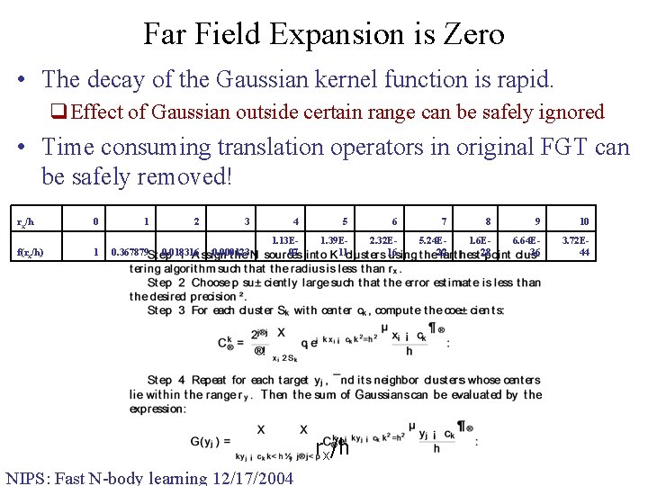
Far Field Expansion is Zero • The decay of the Gaussian kernel function is rapid. q. Effect of Gaussian outside certain range can be safely ignored • Time consuming translation operators in original FGT can be safely removed! rx/h f(rx/h) 0 1 1 0. 367879 2 0. 018316 3 4 5 6 7 8 9 10 0. 000123 1. 13 E 07 1. 39 E 11 2. 32 E 16 5. 24 E 22 1. 6 E 28 6. 64 E 36 3. 72 E 44 rx/h NIPS: Fast N-body learning 12/17/2004

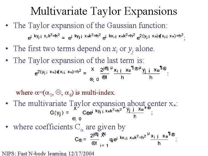
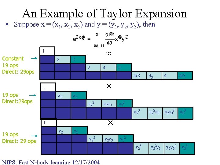
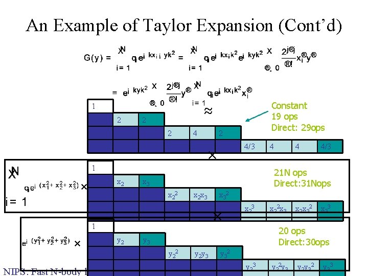
Multivariate Taylor Expansions • The Taylor expansion of the Gaussian function: • The first two terms depend on xi or yj alone. • The Taylor expansion of the last term is: where =( 1, , d) is multi-index. • The multivariate Taylor expansion about center x*: • where coefficients C are given by NIPS: Fast N-body learning 12/17/2004

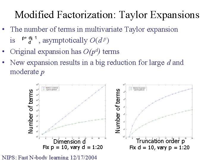
Modified Factorization: Taylor Expansions Number of terms • The number of terms in multivariate Taylor expansion is , asymptotically O(d p) • Original expansion has O(pd) terms • New expansion results in a big reduction for large d and moderate p Dimension d Fix p = 10, vary d = 1: 20 NIPS: Fast N-body learning 12/17/2004 Truncation order p Fix d = 10, vary p = 1: 20

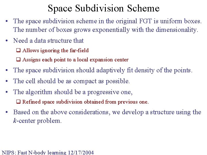
Space Subdivision Scheme • The space subdivision scheme in the original FGT is uniform boxes. The number of boxes grows exponentially with the dimensionality. • Need a data structure that q Allows ignoring the far-field q Assigns each point to a local expansion center • The space subdivision should adaptively fit density of the points. • The cell should be as compact as possible. • The algorithm should be a progressive one, q Refined space subdivision obtained from previous one. • Based on the above considerations, we develop a structure using the k-center problem. NIPS: Fast N-body learning 12/17/2004

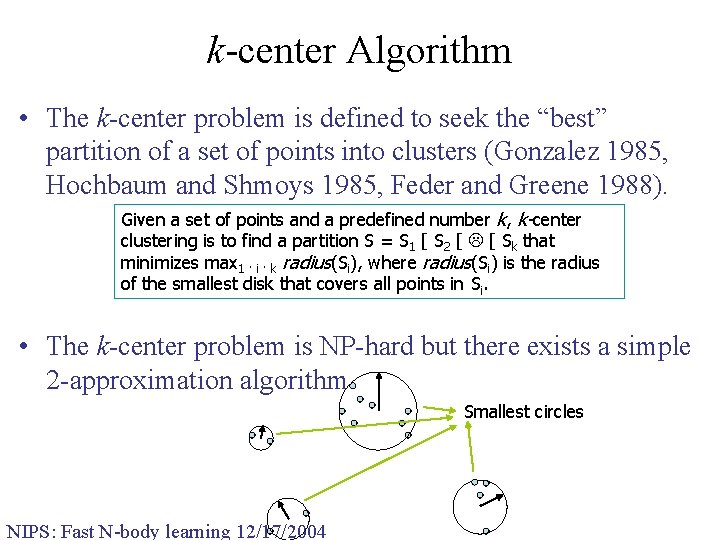
k-center Algorithm • The k-center problem is defined to seek the “best” partition of a set of points into clusters (Gonzalez 1985, Hochbaum and Shmoys 1985, Feder and Greene 1988). Given a set of points and a predefined number k, k-center clustering is to find a partition S = S 1 [ S 2 [ [ Sk that minimizes max 1 · i · k radius(Si), where radius(Si) is the radius of the smallest disk that covers all points in Si. • The k-center problem is NP-hard but there exists a simple 2 -approximation algorithm. Smallest circles NIPS: Fast N-body learning 12/17/2004

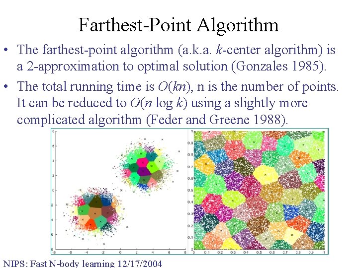
Farthest-Point Algorithm • The farthest-point algorithm (a. k-center algorithm) is a 2 -approximation to optimal solution (Gonzales 1985). • The total running time is O(kn), n is the number of points. It can be reduced to O(n log k) using a slightly more complicated algorithm (Feder and Greene 1988). NIPS: Fast N-body learning 12/17/2004

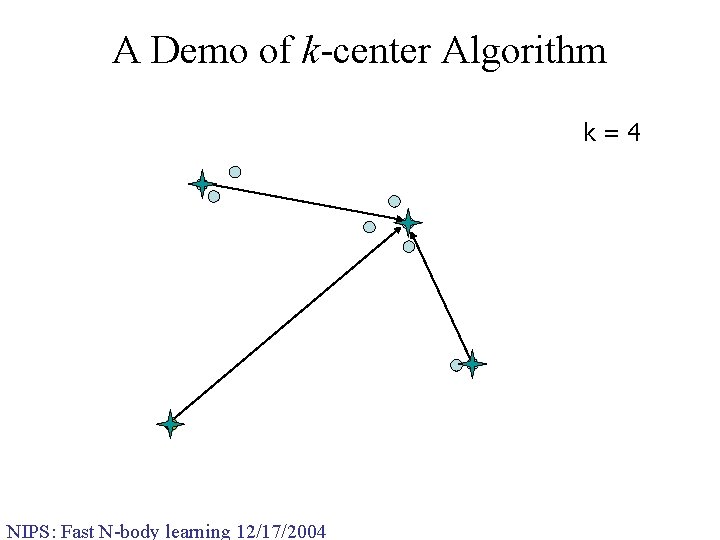
A Demo of k-center Algorithm k=4 NIPS: Fast N-body learning 12/17/2004

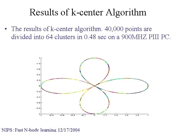
Results of k-center Algorithm • The results of k-center algorithm. 40, 000 points are divided into 64 clusters in 0. 48 sec on a 900 MHZ PIII PC. NIPS: Fast N-body learning 12/17/2004

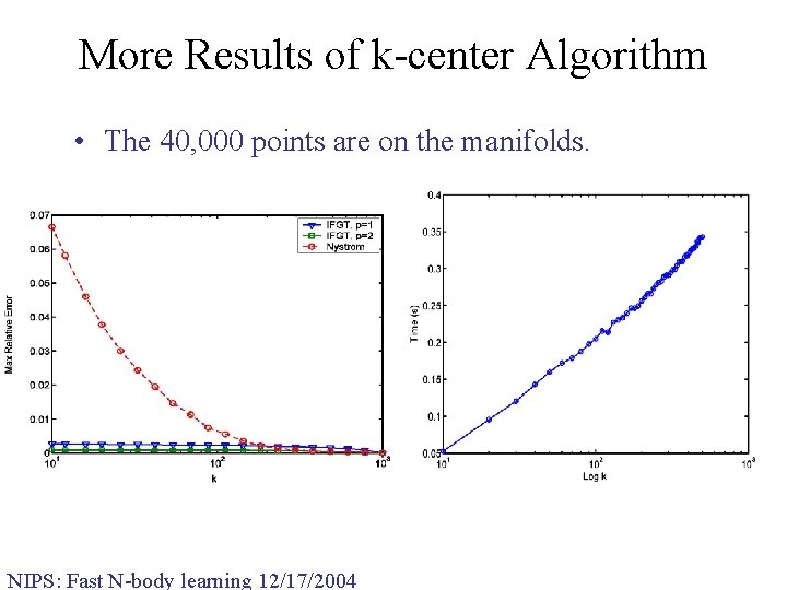
More Results of k-center Algorithm • The 40, 000 points are on the manifolds. NIPS: Fast N-body learning 12/17/2004

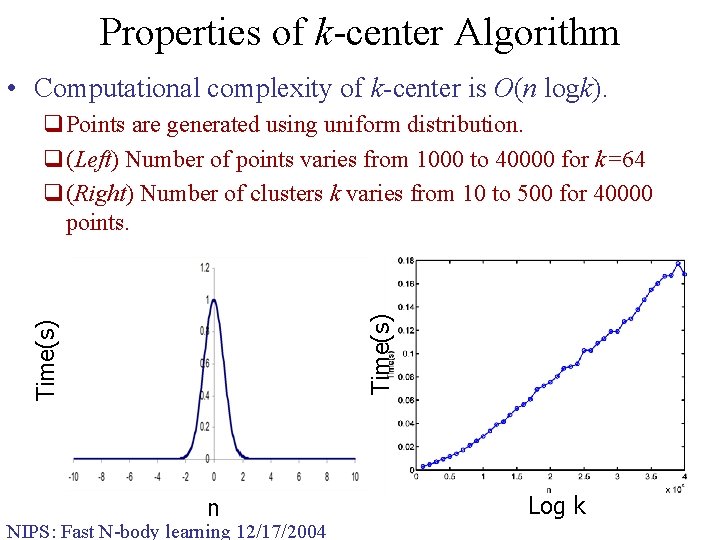
Properties of k-center Algorithm • Computational complexity of k-center is O(n logk). Time(s) q. Points are generated using uniform distribution. q(Left) Number of points varies from 1000 to 40000 for k=64 q(Right) Number of clusters k varies from 10 to 500 for 40000 points. n NIPS: Fast N-body learning 12/17/2004 Log k

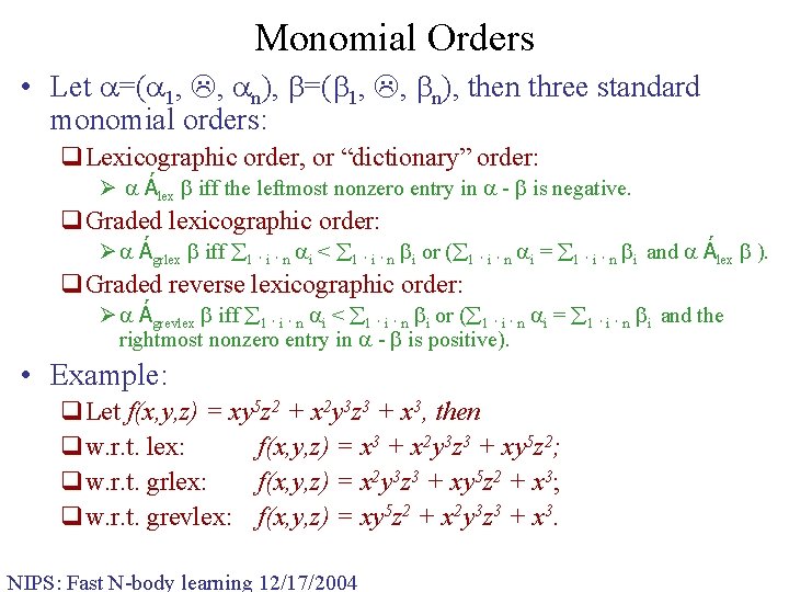
Monomial Orders • Let =( 1, , n), then three standard monomial orders: q. Lexicographic order, or “dictionary” order: Ø Álex iff the leftmost nonzero entry in - is negative. q. Graded lexicographic order: Ø Ágrlex iff 1 · i · n i < 1 · i · n i or ( 1 · i · n i = 1 · i · n i and Álex ). q. Graded reverse lexicographic order: Ø Ágrevlex iff 1 · i · n i < 1 · i · n i or ( 1 · i · n i = 1 · i · n i and the rightmost nonzero entry in - is positive). • Example: q. Let f(x, y, z) = xy 5 z 2 + x 2 y 3 z 3 + x 3, then qw. r. t. lex: f(x, y, z) = x 3 + x 2 y 3 z 3 + xy 5 z 2; qw. r. t. grlex: f(x, y, z) = x 2 y 3 z 3 + xy 5 z 2 + x 3; qw. r. t. grevlex: f(x, y, z) = xy 5 z 2 + x 2 y 3 z 3 + x 3. NIPS: Fast N-body learning 12/17/2004

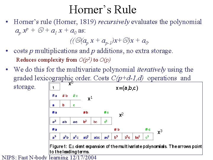
Horner’s Rule • Horner’s rule (Horner, 1819) recursively evaluates the polynomial ap xp + + a 1 x + a 0 as: (( (ap x + ap-1)x+ )x + a 0. • costs p multiplications and p additions, no extra storage. Reduces complexity from O(p 2) to O(p) • We do this for the multivariate polynomial iteratively using the graded lexicographic 0 order. Costs C(p+d-1, d) operations and x storage. x=(a, b, c) x 1 x 2 x 3 NIPS: Fast N-body learning 12/17/2004

An Example of Taylor Expansion • Suppose x = (x 1, x 2, x 3) and y = (y 1, y 2, y 3), then 1 ≈ Constant 19 ops Direct: 29 ops 2 2 4 4 2 4/3 4 4 4 8 4 x 1 x 2 x 3 x 12 x 1 x 3 x 22 x 2 x 3 x 12 x 2 x 12 x 3 x 1 x 22 x 1 x 2 x x 1 x 32 3 1 19 ops Direct: 29 ops 43 4 4/3 x 22 x 3 x 2 x 32 x 33 × 1 19 ops Direct: 29 ops 4/3 x 32 × y 1 y 2 y 3 y 12 y 1 y 3 y 22 y 2 y 3 y 12 y 2 y 12 y 3 y 1 y 22 y 1 y 2 y y 1 y 32 3 NIPS: Fast N-body learning 12/17/2004 y 32 y 23 y 22 y 3 y 2 y 32 y 33

An Example of Taylor Expansion (Cont’d) 1 Constant 19 ops Direct: 29 ops ≈ 2 2 4 4 2 4/3 4 4 4 8 4 × 4/3 1 × x 1 x 2 x 3 x 12 x 1 x 3 x 22 x 2 x 3 x 12 x 2 x 12 x 3 x 1 x 22 x 1 x 2 x x 1 x 32 1 4/3 x 32 × x 23 x 22 x 3 x 2 x 32 x 33 20 ops Direct: 30 ops y 1 y 2 y 3 y 12 y 1 y 3 y 22 y 2 y 3 y 12 y 2 y 12 y 3 y 1 y 22 y 1 y 2 y y 1 y 32 NIPS: Fast N-body learning 12/17/2004 4 21 N ops Direct: 31 Nops 3 × 4 y 32 y 23 y 22 y 3 y 2 y 32 y 33

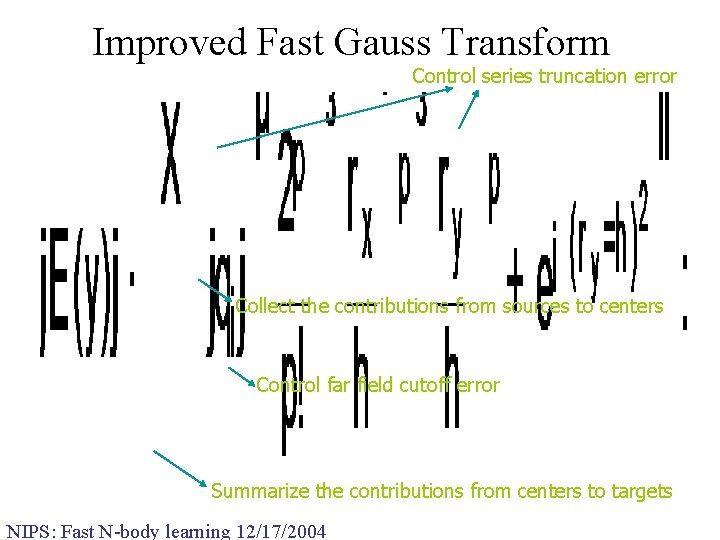
Improved Fast Gauss Transform Control series truncation error Collect the contributions from sources to centers Control far field cutoff error Summarize the contributions from centers to targets NIPS: Fast N-body learning 12/17/2004

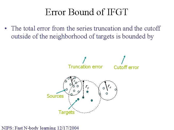
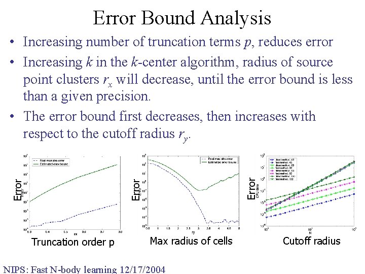
Error Bound of IFGT • The total error from the series truncation and the cutoff outside of the neighborhood of targets is bounded by Truncation error Cutoff error rx ry Sources Targets NIPS: Fast N-body learning 12/17/2004 rx

Error Bound Analysis Error • Increasing number of truncation terms p, reduces error • Increasing k in the k-center algorithm, radius of source point clusters rx will decrease, until the error bound is less than a given precision. • The error bound first decreases, then increases with respect to the cutoff radius ry. Truncation order p Max radius of cells NIPS: Fast N-body learning 12/17/2004 Cutoff radius

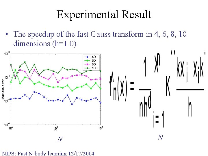
Experimental Result • The speedup of the fast Gauss transform in 4, 6, 8, 10 dimensions (h=1. 0). N NIPS: Fast N-body learning 12/17/2004 N

Efficient Kernel Density Estimation NIPS: Fast N-body learning 12/17/2004

Kernel Density Estimation (KDE) • Kernel density estimation (a. k. a Parzen method, Rosenblatt 1956, Parzen 1962) is an important nonparametric technique. • KDE is the keystone of many algorithms: q. Radial basis function networks q. Support vector machines q. Mean shift algorithm q. Regularized particle filter • The main drawback is the quadratic computational complexity. Very slow for large dataset. NIPS: Fast N-body learning 12/17/2004

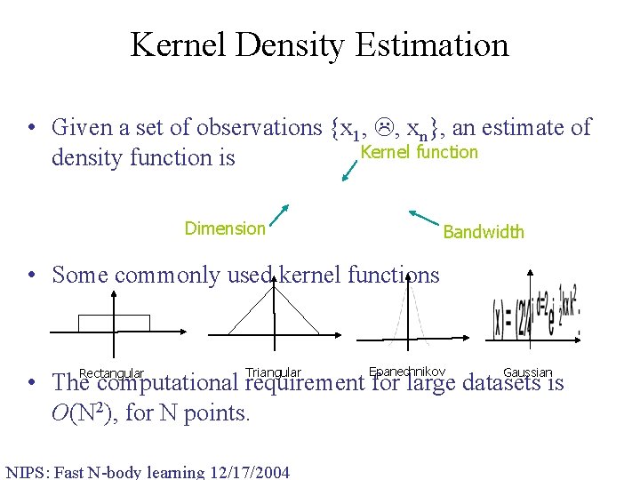
Kernel Density Estimation • Given a set of observations {x 1, , xn}, an estimate of Kernel function density function is Dimension Bandwidth • Some commonly used kernel functions Rectangular Triangular Epanechnikov Gaussian • The computational requirement for large datasets is O(N 2), for N points. NIPS: Fast N-body learning 12/17/2004

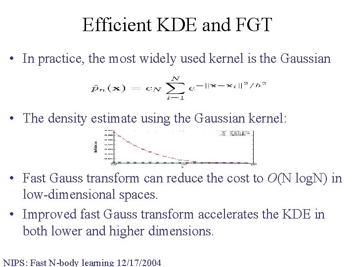
Efficient KDE and FGT • In practice, the most widely used kernel is the Gaussian • The density estimate using the Gaussian kernel: • Fast Gauss transform can reduce the cost to O(N log. N) in low-dimensional spaces. • Improved fast Gauss transform accelerates the KDE in both lower and higher dimensions. NIPS: Fast N-body learning 12/17/2004

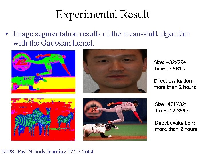
Experimental Result • Image segmentation results of the mean-shift algorithm with the Gaussian kernel. Size: 432 X 294 Time: 7. 984 s Direct evaluation: more than 2 hours Size: 481 X 321 Time: 12. 359 s Direct evaluation: more than 2 hours NIPS: Fast N-body learning 12/17/2004

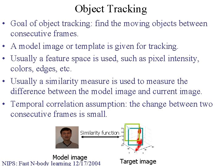
Object Tracking • Goal of object tracking: find the moving objects between consecutive frames. • A model image or template is given for tracking. • Usually a feature space is used, such as pixel intensity, colors, edges, etc. • Usually a similarity measure is used to measure the difference between the model image and current image. • Temporal correlation assumption: the change between two consecutive frames is small. Similarity function Model image NIPS: Fast N-body learning 12/17/2004 Target image

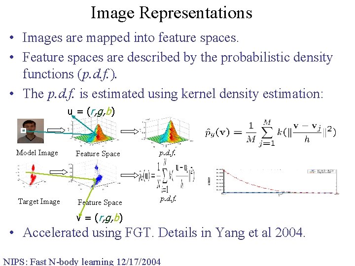
Image Representations • Images are mapped into feature spaces. • Feature spaces are described by the probabilistic density functions (p. d. f. ). • The p. d. f. is estimated using kernel density estimation: u = (r, g, b) Model Image Feature Space Target Image Feature Space p. d. f. v = (r, g, b) • Accelerated using FGT. Details in Yang et al 2004. NIPS: Fast N-body learning 12/17/2004

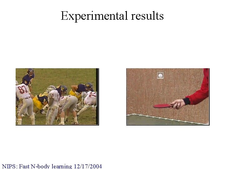
Experimental results NIPS: Fast N-body learning 12/17/2004

Regularized Least Squares Classification • RLSC is a regularized least-squares based perceptron q. Only need to solve linear systems q. Use square-loss regularization (Poggio 1989, Wahba 1990) q. Comparable accuracy with the SVMs • Three variants of RLSC q 1999, Hans Suykens, Least Squares SVM q 2001, Fung & Mangasarian, Proximal SVM q 2002, Rifkin & Poggio, RLSC NIPS: Fast N-body learning 12/17/2004

The RLSC Algorithm NIPS: Fast N-body learning 12/17/2004

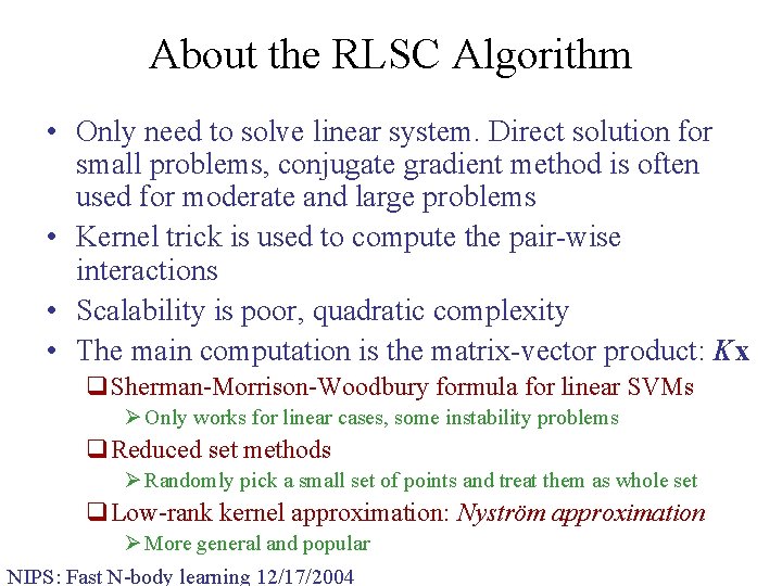
About the RLSC Algorithm • Only need to solve linear system. Direct solution for small problems, conjugate gradient method is often used for moderate and large problems • Kernel trick is used to compute the pair-wise interactions • Scalability is poor, quadratic complexity • The main computation is the matrix-vector product: Kx q. Sherman-Morrison-Woodbury formula for linear SVMs Ø Only works for linear cases, some instability problems q. Reduced set methods Ø Randomly pick a small set of points and treat them as whole set q. Low-rank kernel approximation: Nyström approximation Ø More general and popular NIPS: Fast N-body learning 12/17/2004

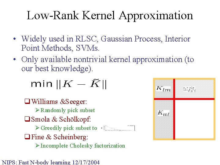
Low-Rank Kernel Approximation • Widely used in RLSC, Gaussian Process, Interior Point Methods, SVMs. • Only available nontrivial kernel approximation (to our best knowledge). q. Williams &Seeger: Ø Randomly pick subset q. Smola & Schölkopf: Ø Greedily pick subset to q. Fine & Scheinberg: Ø Incomplete Cholesky factorization NIPS: Fast N-body learning 12/17/2004

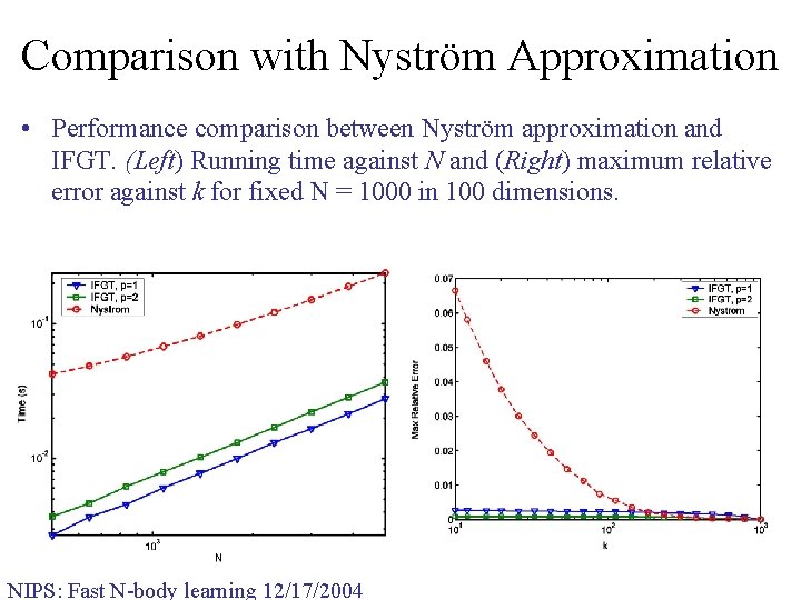
Comparison with Nyström Approximation • Performance comparison between Nyström approximation and IFGT. (Left) Running time against N and (Right) maximum relative error against k for fixed N = 1000 in 100 dimensions. NIPS: Fast N-body learning 12/17/2004

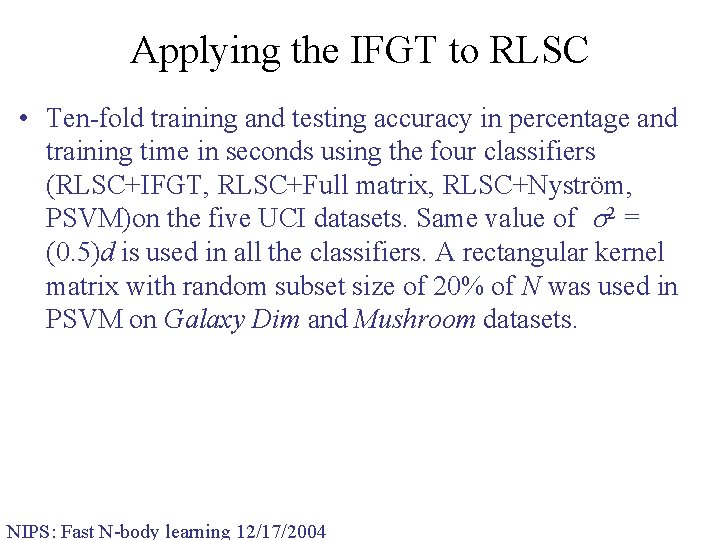
Applying the IFGT to RLSC • Ten-fold training and testing accuracy in percentage and training time in seconds using the four classifiers (RLSC+IFGT, RLSC+Full matrix, RLSC+Nyström, PSVM)on the five UCI datasets. Same value of 2 = (0. 5)d is used in all the classifiers. A rectangular kernel matrix with random subset size of 20% of N was used in PSVM on Galaxy Dim and Mushroom datasets. NIPS: Fast N-body learning 12/17/2004

Applying the IFGT to RLSC (Cont’d) NIPS: Fast N-body learning 12/17/2004

Code • FGT code FIGTREE (v 1. 0) released q. Free for noncommercial use q. Send email to yangcj@cs. umd. edu to get license. Accept the license and we mail you the code. NIPS: Fast N-body learning 12/17/2004