Fast Multipole Method for Multiparticle Simulations He Zhang

Fast Multipole Method for Multiparticle Simulations He Zhang ICAP’ 18 10/21/2018 Key West, FL, USA

Introduction of FMM o A fast algorithm to calculate the interaction among N particles. o Basic idea of FMM o the kernel can be represented by expansions that converges with distance. o Group the particles by their positions o Near region interaction is calculated directly by the pairwise formula o Far region interaction is calculated by the multipole/local expansion o Property of FMM o Gridless o Scales O(N) for non-oscillatory kernel with open boundary, and O(Nlog. N) for oscillatory kernel with open boundary. o Accuracy is determined only by the order/rank of the expansions and the error can be strictly estimated and controlled. o Can be combined with other methods to solve boundary value problem. o FMM is widely used in electric engineering, mechanic engineering, biophysics, etc. But not yet in accelerator/beam physics. He Zhang ---2 ---

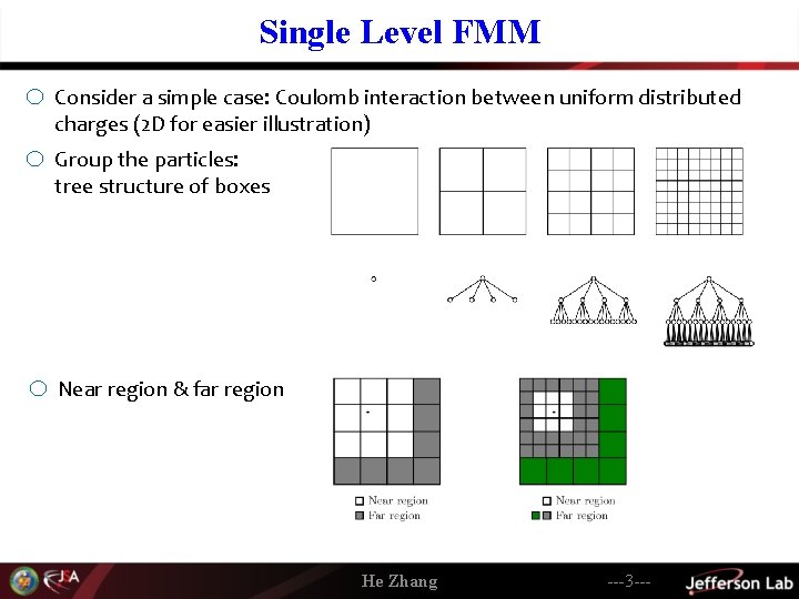
Single Level FMM o Consider a simple case: Coulomb interaction between uniform distributed charges (2 D for easier illustration) o Group the particles: tree structure of boxes o Near region & far region He Zhang ---3 ---

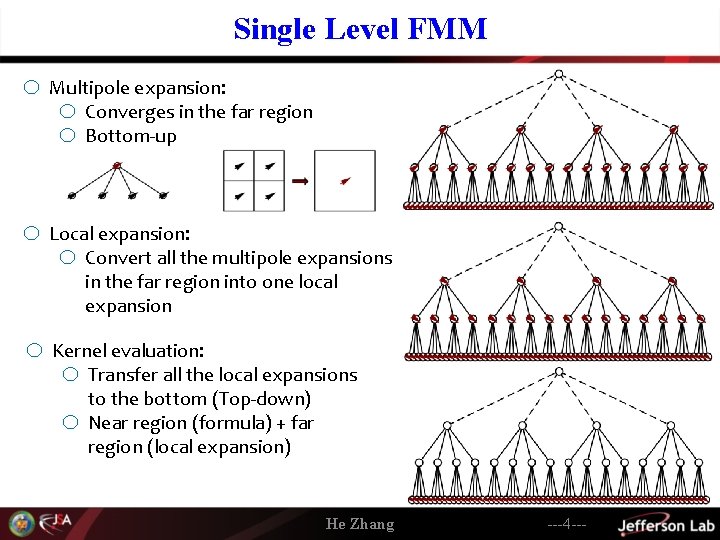
Single Level FMM o Multipole expansion: o Converges in the far region o Bottom-up o Local expansion: o Convert all the multipole expansions in the far region into one local expansion o Kernel evaluation: o Transfer all the local expansions to the bottom (Top-down) o Near region (formula) + far region (local expansion) He Zhang ---4 ---

Single Level FMM o Four steps procedure of FMM 1. Decompose the space hierarchically into boxes of tree structure 2. Going up the tree to calculate the multipole expansions in all the boxes 3. Going down the tree to calculate the local expansions in all the boxes 4. Calculate the potential/field inside the lowest level boxes o How about non-uniform distributions? He Zhang ---5 ---

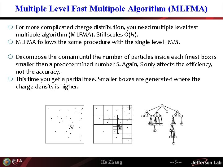
Multiple Level Fast Multipole Algorithm (MLFMA) o For more complicated charge distribution, you need multiple level fast multipole algorithm (MLFMA). Still scales O(N). o MLFMA follows the same procedure with the single level FMM. o Decompose the domain until the number of particles inside each finest box is o smaller than a predetermined number S. Again, S only affects the efficiency, not the accuracy. This time you get a partial tree. Smaller boxes are generated where the charge density is higher. He Zhang ---6 ---

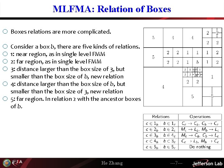
MLFMA: Relation of Boxes o Boxes relations are more complicated. o Consider a box b, there are five kinds of relations. o 1: near region, as in single level FMM o 2: far region, as in single level FMM o 3: distance larger than the box size of 3, but smaller than the box size of b, new relation o 4: distance larger than the box size of b, but smaller than the box size of 3, new relation o 5: far region. In relation 2 with the ancestor boxes of b. He Zhang ---7 ---

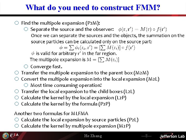
What do you need to construct FMM? o Find the multipole expansion (P 2 M): o Separate the source and the observer: o Converge fast. o Transfer the multipole expansion to the parent box (M 2 M) o Convert the multipole expansion into the local expansion (M 2 L) o Most time consuming operation! o Transfer the local expansion to the child boxes (L 2 L) o Calculate the kernel by the local expansion (L 2 P) o Calculate the kernel by the formula (P 2 P) Another two formulas for MLFMA Calculate the local expansion by source particles (P 2 L) Calculate the kernel by multipole expansion (M 2 P) o o He Zhang ---8 ---

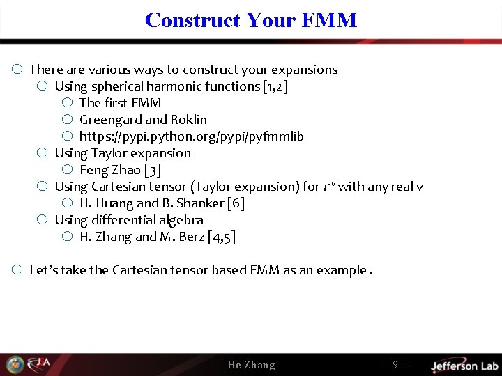
Construct Your FMM o There are various ways to construct your expansions o Using spherical harmonic functions [1, 2] o The first FMM o Greengard and Roklin o https: //pypi. python. org/pypi/pyfmmlib o Using Taylor expansion o Feng Zhao [3] o Using Cartesian tensor (Taylor expansion) for r-v with any real v o H. Huang and B. Shanker [6] o Using differential algebra o H. Zhang and M. Berz [4, 5] o Let’s take the Cartesian tensor based FMM as an example. He Zhang ---9 ---

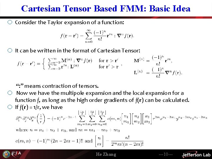
Cartesian Tensor Based FMM: Basic Idea o Consider the Taylor expansion of a function: o It can be written in the format of Cartesian Tensor: o o “: ” means contraction of tensors. Now we have the multipole expansion and the local expansion for a function f, as long as the high order gradients of f(r) can be calculated. If f(r) = 1/r, we have He Zhang ---10 ---

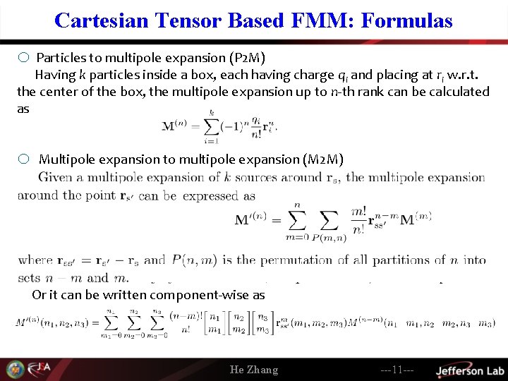
Cartesian Tensor Based FMM: Formulas o Particles to multipole expansion (P 2 M) Having k particles inside a box, each having charge qi and placing at ri w. r. t. the center of the box, the multipole expansion up to n-th rank can be calculated as o Multipole expansion to multipole expansion (M 2 M) Or it can be written component-wise as He Zhang ---11 ---

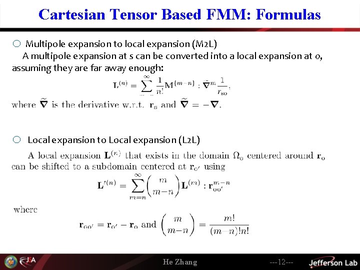
Cartesian Tensor Based FMM: Formulas o Multipole expansion to local expansion (M 2 L) A multipole expansion at s can be converted into a local expansion at o, assuming they are far away enough: o Local expansion to Local expansion (L 2 L) He Zhang ---12 ---

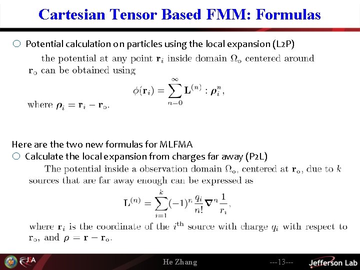
Cartesian Tensor Based FMM: Formulas o Potential calculation on particles using the local expansion (L 2 P) Here are the two new formulas for MLFMA Calculate the local expansion from charges far away (P 2 L) o He Zhang ---13 ---

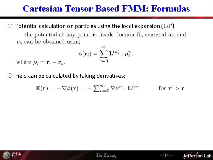
Cartesian Tensor Based FMM: Formulas o Potential calculation on particles using the local expansion (L 2 P) o Field can be calculated by taking derivatives: He Zhang ---14 ---

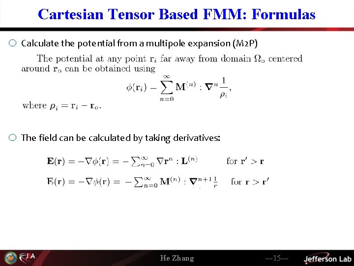
Cartesian Tensor Based FMM: Formulas o Calculate the potential from a multipole expansion (M 2 P) o The field can be calculated by taking derivatives: He Zhang ---15 ---

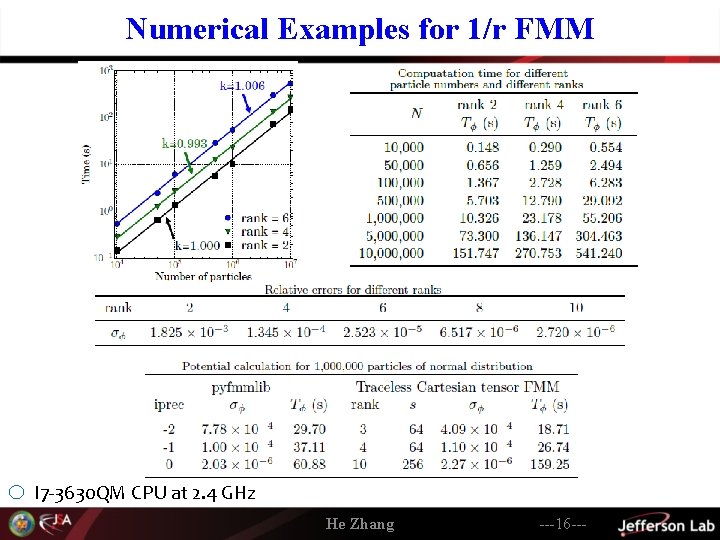
Numerical Examples for 1/r FMM o I 7 -3630 QM CPU at 2. 4 GHz He Zhang ---16 ---

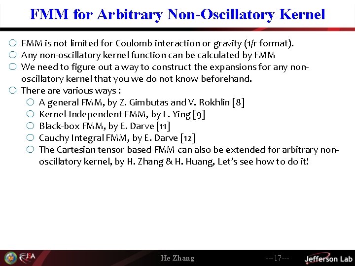
FMM for Arbitrary Non-Oscillatory Kernel o FMM is not limited for Coulomb interaction or gravity (1/r format). o Any non-oscillatory kernel function can be calculated by FMM o We need to figure out a way to construct the expansions for any nonoscillatory kernel that you we do not know beforehand. o There are various ways : o A general FMM, by Z. Gimbutas and V. Rokhlin [8] o Kernel-Independent FMM, by L. Ying [9] o Black-box FMM, by E. Darve [11] o Cauchy Integral FMM, by E. Darve [12] o The Cartesian tensor based FMM can also be extended for arbitrary nonoscillatory kernel, by H. Zhang & H. Huang, Let’s see how to do it! He Zhang ---17 ---

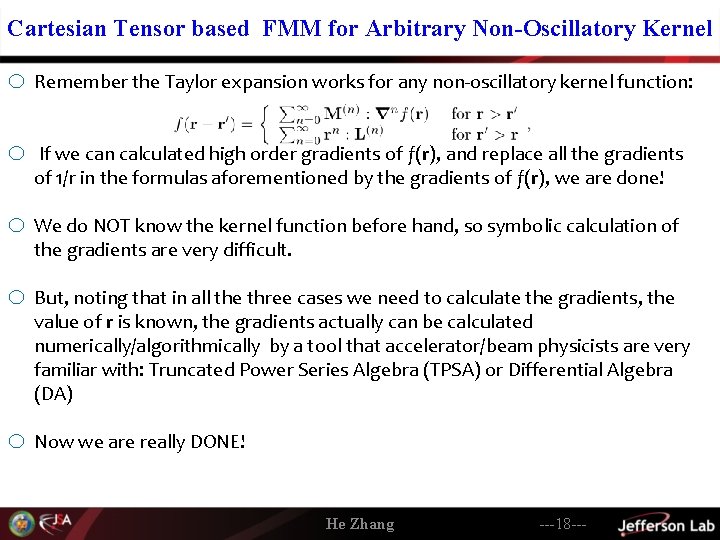
Cartesian Tensor based FMM for Arbitrary Non-Oscillatory Kernel o Remember the Taylor expansion works for any non-oscillatory kernel function: o If we can calculated high order gradients of f(r), and replace all the gradients of 1/r in the formulas aforementioned by the gradients of f(r), we are done! o We do NOT know the kernel function before hand, so symbolic calculation of the gradients are very difficult. o But, noting that in all the three cases we need to calculate the gradients, the value of r is known, the gradients actually can be calculated numerically/algorithmically by a tool that accelerator/beam physicists are very familiar with: Truncated Power Series Algebra (TPSA) or Differential Algebra (DA) o Now we are really DONE! He Zhang ---18 ---

Parallelization of FMM o o Parallelization of MLFMA is very challenging due to the unbalanced partial tree. Fortunately, great efforts have been put to solve this problem, with great achievements. Now MLFMA parallelizes well on thousands or even more of nodes Some libraries: Pyfmmlib: Python interface with Fortran code underneath. https: //pypi. python. org/pypi/pyfmmlib Parallel via Open. MP (shared memory) PVFMM Parallel kernel-independent fmm via MPI (distributed structure) https: //github. com/dmalhotra/pvfmm Blood flow simulation, 90 billion unknowns simulated in each step tiem, won 2010 Gordon Bell Prize, parallel on 200, 000 AMD notes on ORNL Jaguar PF system [10] (pkifmm) Exafmm Supporting various kernels Excellent parallel scaling via MPI (distributed structure) https: //github. com/exafmm The author won Gordon Bell prize in 2009 [13] In July 2011, field of 3, 011, 561, 968, 121 particles are calculated in 11 mins, JSC, Germany o o o o He Zhang ---19 ---

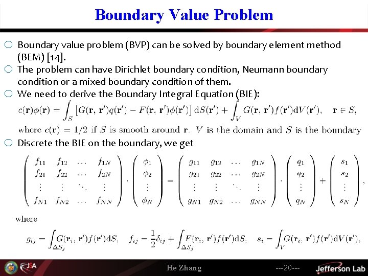
Boundary Value Problem o Boundary value problem (BVP) can be solved by boundary element method (BEM) [14]. o The problem can have Dirichlet boundary condition, Neumann boundary condition or a mixed boundary condition of them. o We need to derive the Boundary Integral Equation (BIE): o Discrete the BIE on the boundary, we get He Zhang ---20 ---

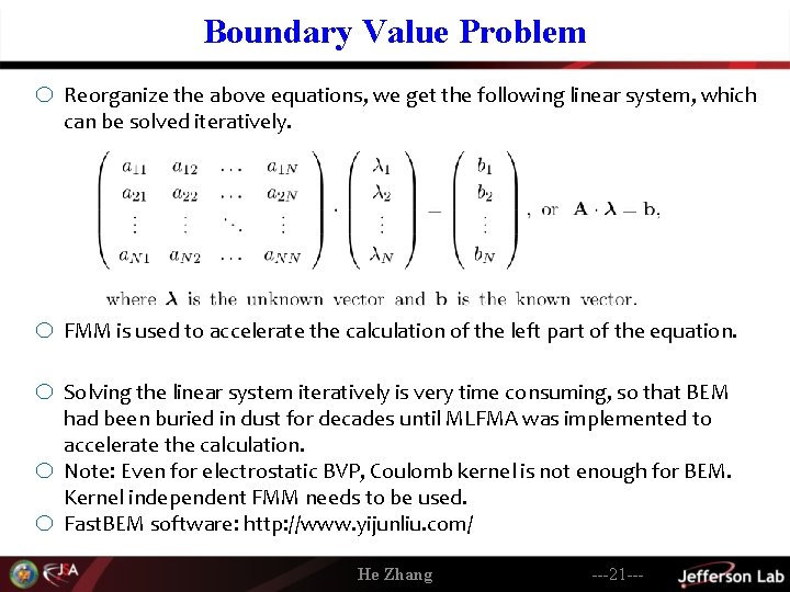
Boundary Value Problem o Reorganize the above equations, we get the following linear system, which can be solved iteratively. o FMM is used to accelerate the calculation of the left part of the equation. o Solving the linear system iteratively is very time consuming, so that BEM o o had been buried in dust for decades until MLFMA was implemented to accelerate the calculation. Note: Even for electrostatic BVP, Coulomb kernel is not enough for BEM. Kernel independent FMM needs to be used. Fast. BEM software: http: //www. yijunliu. com/ He Zhang ---21 ---

Use FMM in Accelerator Study o Particle-In-Cell (PIC) is the dominating algorithm of multi-particle simulation for accelerator studies. o FMM could be a complementary algorithm o FMM is gridless: o Works for any charge distribution and any geometry. o No redundant calculation on the grid points in free space. o Near region is calculated accurately by formula. o Use a library is possible. o But make sure you understand what it calculates and revise it to fit your problem if necessary! He Zhang ---22 ---

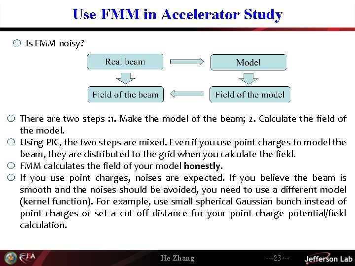
Use FMM in Accelerator Study o Is FMM noisy? o There are two steps : 1. Make the model of the beam; 2. Calculate the field of the model. o Using PIC, the two steps are mixed. Even if you use point charges to model the beam, they are distributed to the grid when you calculate the field. o FMM calculates the field of your model honestly. o If you use point charges, noises are expected. If you believe the beam is smooth and the noises should be avoided, you need to use a different model (kernel function). For example, use small spherical Gaussian bunch instead of point charges or set a cut off distance for your point charge potential/field calculation. He Zhang ---23 ---

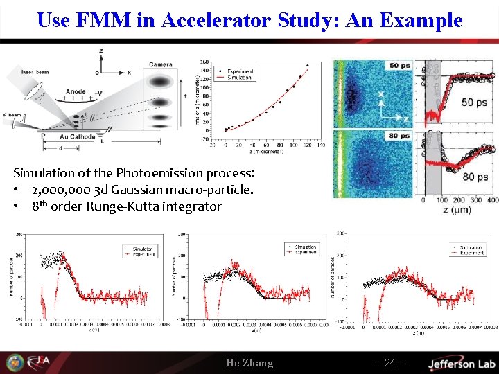
Use FMM in Accelerator Study: An Example Simulation of the Photoemission process: • 2, 000 3 d Gaussian macro-particle. • 8 th order Runge-Kutta integrator He Zhang ---24 ---

Use FMM in Accelerator Study: Other Attempts o Prof. Martin Berz’s group at Michigan State University: o space charge effect in photoemission process o Prof. Bela Erldelyi’s group at Northern Illinois University: o BVP o Electron cooling o http: //niu. edu/beamphysicscode/ o Prof. Pavel Snopok at Illinois Institute of Technology: o Space charge effect in ionization cooling o Prof. Yue Hao at Michigan State University: o Beam-beam effect o Dr. He huang and Dr. He Zhang at Jefferson Lab: o FMM based algorithm development & implementation He Zhang ---25 ---

Oscillatory Kernel o FMM can be used to solve electromagnetic problem in the frequency domain (Helmholtz equation). Computation scales O(Nlog. N). [7, 15, 20] o Implementation is different with non-oscillatory kernel, but it shares the o o o same idea: find the representation that converges fast and separate the sources and the objects. Problems with a general oscillatory kernel can be solved by Kernel Independent FMM + Fast directional method, by L. Ying [16] Black-box FMM + Fast directional method, by E. Darve [17] Boundary value problem can be solved by combining FMM with Combined Field Integral Equation (CFIE). [18] https: //sourceforge. net/projects/puma-em/? source=navbar Parallel via MPI Electromagnetic problem in time domain remains an open question, although there are some works on this topic [19]. o o He Zhang ---26 ---

Summary o FMM is a powerful tool to calculate the pairwise interaction between particles. o Scales linearly with the number of particles. o Grid-independent and suitable for complicated charge distribution and geometry. o Can treat arbitrary non-oscillatory problem and oscillatory problem in frequency domain. o Besides the open boundary problem, FMM can solve BVP if combined with BEM. o High efficiency open source parallel FMM packages have been developed. o Could be a useful tool for multiparticle simulations in accelerator study. He Zhang ---27 ---

He Zhang --28 --

References 1. A fast adaptive multipole algorithm for particle simulations, J Carrier, L Greengard, V Rokhlin, SIAM journal on scientific and statistical computing 9 (4), 1988 2. A fast Adaptive Multipole Algorithm in Three Dimensions, H. Cheng, L. Greengard, and V. Rokhlin, Journal of computational physics 155. 2, 1999 3. An O(N) algorithm for three-dimensional n-body simulations, Feng Zhao, MIT master thesis, 1987 4. The fast multipole method in the differential algebra framework, H. Zhang, M. Berz, NIM A, 2011 5. Space charge simulations of photoemission using the differential algebra-based multiple-level fast multipole method, H. Zhang, Z. Tao, C. -Y. Ruan, et. al. , Microscopy and Microanalysis, 21, 224. , 2015 6. Accelerated Cartesian expansion - A fast method for computing of potentials of the form R^-v for all real v, B. Shanker, H. Huang, JCOMP, 2007. 7. A novel wideband FMM for fast integral equation solution of multiscale problems in Electromagnetics, M. Vikram, H. Huang, B. Shanker, T. Van, Transactions on antennas and propagation, 2009 8. A generalized fast multipole method for non-oscillatory kernels, Z. Gimbutas and V. Rokhlin, SIAM Journal on Scientific Computing 24. 3, 2000 He Zhang ---29 ---

References 9. A kernel-independent adaptive fast multipole algorithm in two and three dimensions, Lexing Ying, George Biros, Denis Zorin, JCOMP, 2004 10. Petascale direct numerical simulation of blood flow on 200 K cores and heterogeneous architectures, A. Rahimian, I Lashuk, S Veerapaneni, et al. Proceedings of the 2010 ACM/IEEE International Conference for High Performance Computing, Networking, Storage and Analysis. IEEE Computer Society, 2010 11. The black-box fast multipole method, William Fong, Eric Darve, JCOMP, 2009 12. Fast multipole method using the Cauchy integral formula, C Cecka, P. -D. Letourneau, E. Darve, Numerical Analysis of Multiscale Computations (pp. 127 -144). Springer, Berlin, Heidelberg. , 2012 13. 42 TFlops hierarchical n-body simulations on GPUs with applications in both astrophysics and turbulence, T. Hamada, T. Narumi, R. Yokota, et al. High Performance Computing Networking, Storage and Analysis, Proceedings of the Conference on. IEEE, 2009. 14. Fast multipole accelerated boundary integral equation methods, N Nishimura, Appl. Mech. Rev 55(4), 299 -324, 2002 15. Diagonal forms of translation operators for the Helmholtz equation in three dimensions, V. Rokhlin, Appl. Comput. Harmon. Anal. 1 (1) (1993) 82 -93 16. Fast directional algorithms for the Helmholtz kernel, B. Engquist, L. Ying, Journal of computational and applied mathematics, 2010 He Zhang ---30 ---

References 17. Fast directional multilevel summation for oscillatory kernels based on Chebyshev interpolation, M. Messner, M. Schanz, E. Darve, JCOMP, 2012 18. Fast multipole method solution of three dimensional integral equation, J. M. Song, W. C. Chew, Antennas and Propagation Society International Symposium, 1995. AP-S. Digest. Vol. 3. IEEE, 1995. 19. Fast and Efficient Algorithms in Computational Electromagnetics, W. Chew, E. Michielssen, J. M. Song, J. M. Jin (Eds. ), Artech House, Inc. , Norwood, MA, USA, 2001. 20. A wideband fast multipole method for the Helmholtz equation in three dimensions, H. Cheng, W. Y. Crutchfield, Z. Gimbutas, L. F. Greengard, et al. , J. Comput. Phys. 216 (1) (2006) 300 -325. He Zhang ---31 ---

BACKUP SLIDES He Zhang --32 --

Single Level FMM o Single level FMM works well for uniform charge distribution. o It demonstrate the principle and the procedure of FMM. o It is easier to understand. o For more complicated charge distribution, multiple level fast multipole algorithm (FLFMA) is better, which will be explained later. o Four steps procedure of FMM 1. Decompose the space hierarchically into boxes of tree structure 2. Going up the tree to calculate the multipole expansions in all the boxes 3. Going down the tree to calculate the local expansions in all the boxes 4. Calculate the potential/field inside the lowest level boxes He Zhang ---33 ---

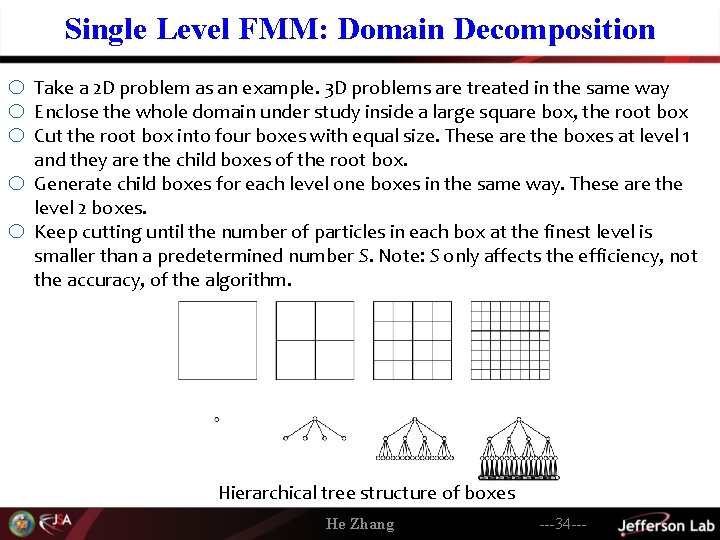
Single Level FMM: Domain Decomposition o Take a 2 D problem as an example. 3 D problems are treated in the same way o Enclose the whole domain under study inside a large square box, the root box o Cut the root box into four boxes with equal size. These are the boxes at level 1 and they are the child boxes of the root box. o Generate child boxes for each level one boxes in the same way. These are the level 2 boxes. o Keep cutting until the number of particles in each box at the finest level is smaller than a predetermined number S. Note: S only affects the efficiency, not the accuracy, of the algorithm. Hierarchical tree structure of boxes He Zhang ---34 ---

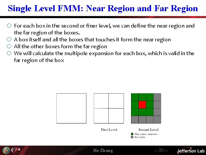
Single Level FMM: Near Region and Far Region o For each box in the second or finer level, we can define the near region and the far region of the boxes. o A box itself and all the boxes that touches it form the near region o All the other boxes form the far region o We will calculate the multipole expansion for each box, which is valid in the far region of the box He Zhang ---35 ---

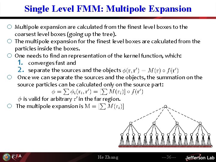
Single Level FMM: Multipole Expansion o Multipole expansion are calculated from the finest level boxes to the coarsest level boxes (going up the tree). o The multipole expansion for the finest level boxes are calculated from the particles inside the boxes. o One needs to find an representation of the kernel function, which: 1. converges fast and 2. separate the sources and the objects o Once we can separate the sources and the objects, the summation on the source particles can be calculated only on the source part: o is valid for arbitrary in the far region. The multipole expansion is He Zhang ---36 ---

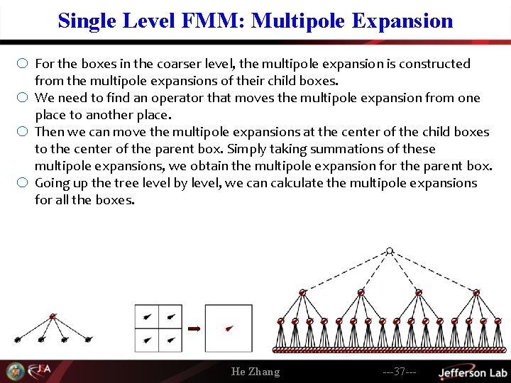
Single Level FMM: Multipole Expansion o For the boxes in the coarser level, the multipole expansion is constructed from the multipole expansions of their child boxes. o We need to find an operator that moves the multipole expansion from one place to another place. o Then we can move the multipole expansions at the center of the child boxes o to the center of the parent box. Simply taking summations of these multipole expansions, we obtain the multipole expansion for the parent box. Going up the tree level by level, we can calculate the multipole expansions for all the boxes. He Zhang ---37 ---

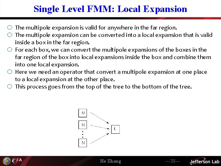
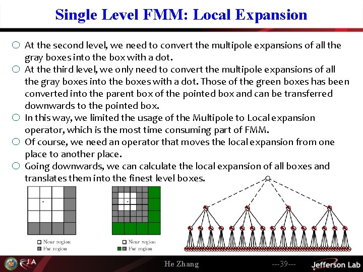
Single Level FMM: Local Expansion o The multipole expansion is valid for anywhere in the far region. o The multipole expansion can be converted into a local expansion that is valid inside a box in the far region. o For each box, we can convert the multipole expansions of the boxes in the o o far region of the box into local expansions inside the box and combine them into one local expansion. Here we need an operator that convert a multipole expansion at one place to a local expansion at the other place. This process goes from the top of the tree to the bottom of the tree. He Zhang ---38 ---

Single Level FMM: Local Expansion o At the second level, we need to convert the multipole expansions of all the gray boxes into the box with a dot. o At the third level, we only need to convert the multipole expansions of all o o o the gray boxes into the boxes with a dot. Those of the green boxes has been converted into the parent box of the pointed box and can be transferred downwards to the pointed box. In this way, we limited the usage of the Multipole to Local expansion operator, which is the most time consuming part of FMM. Of course, we need an operator that moves the local expansion from one place to another place. Going downwards, we can calculate the local expansion of all boxes and translates them into the finest level boxes. He Zhang ---39 ---

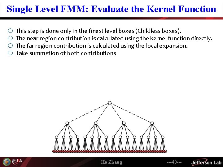
Single Level FMM: Evaluate the Kernel Function o This step is done only in the finest level boxes (Childless boxes). o The near region contribution is calculated using the kernel function directly. o The far region contribution is calculated using the local expansion. o Take summation of both contributions He Zhang ---40 ---

Single Level FMM: An Implemetation o There are various ways to construct your expansions o Using spherical harmonic functions [1, 2] o The first FMM o Greengard and Roklin o https: //pypi. python. org/pypi/pyfmmlib o Using Taylor expansion o Feng Zhao [3] o Using Cartesian tensor (Taylor expansion) for r-v with any real v o H. Huang and B. Shanker [6] o Using differential algebra o H. Zhang and M. Berz [4, 5] o Let’s take the Cartesian tensor based FMM as an example to see how to construct the multipole expansions and the local expansions. o The Cartesian tensor based FMM is straightforward and the math may be less scary to beginners. He Zhang ---41 ---