Fast integration using quasirandom numbers J Bossert M

Fast integration using quasi-random numbers J. Bossert, M. Feindt, U. Kerzel University of Karlsruhe ACAT 05 xx May 2005 Ulrich Kerzel, University of Karlsruhe, ACAT 05 - Zeuthen

Outline l l Numerical integration Discrepancy l l Pseudo- and quasi-random numbers l l l The Koksma-Hlawka inequality Generators for quasi-random numbers Optimising the discrepancy Quasi-random numbers in n dimensions Comparison Examples xx May 2005 Ulrich Kerzel, University of Karlsruhe, ACAT 05 - Zeuthen 2

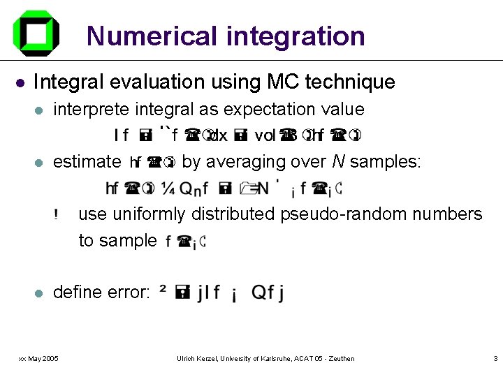
Numerical integration l Integral evaluation using MC technique l interprete integral as expectation value l estimate by averaging over N samples: use uniformly distributed pseudo-random numbers to sample l define error: xx May 2005 Ulrich Kerzel, University of Karlsruhe, ACAT 05 - Zeuthen 3

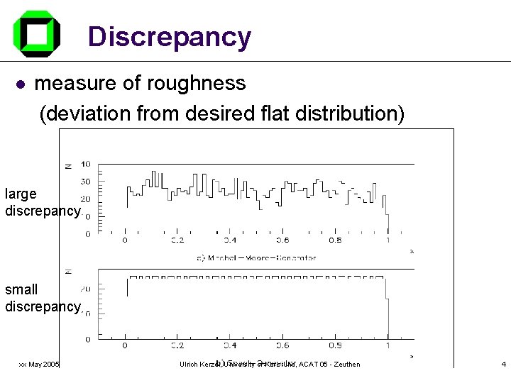
Discrepancy l measure of roughness (deviation from desired flat distribution) large discrepancy small discrepancy xx May 2005 Ulrich Kerzel, University of Karlsruhe, ACAT 05 - Zeuthen 4

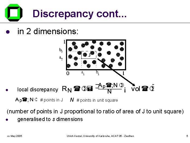
Discrepancy cont. . . l in 2 dimensions: l local discrepancy # points in J N # points in unit square (number of points in J proportional to ratio of area of J to unit square) l generalised to s dimensions xx May 2005 Ulrich Kerzel, University of Karlsruhe, ACAT 05 - Zeuthen 5

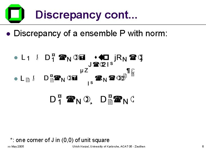
Discrepancy cont. . . l Discrepancy of a ensemble P with norm: l l *: one corner of J in (0, 0) of unit square xx May 2005 Ulrich Kerzel, University of Karlsruhe, ACAT 05 - Zeuthen 6

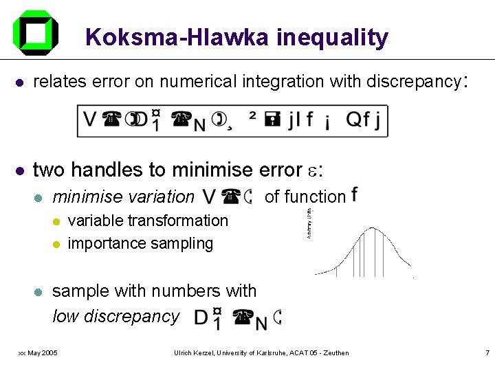
Koksma-Hlawka inequality l relates error on numerical integration with discrepancy: l two handles to minimise error : l minimise variation l l l of function variable transformation importance sampling sample with numbers with low discrepancy xx May 2005 Ulrich Kerzel, University of Karlsruhe, ACAT 05 - Zeuthen 7

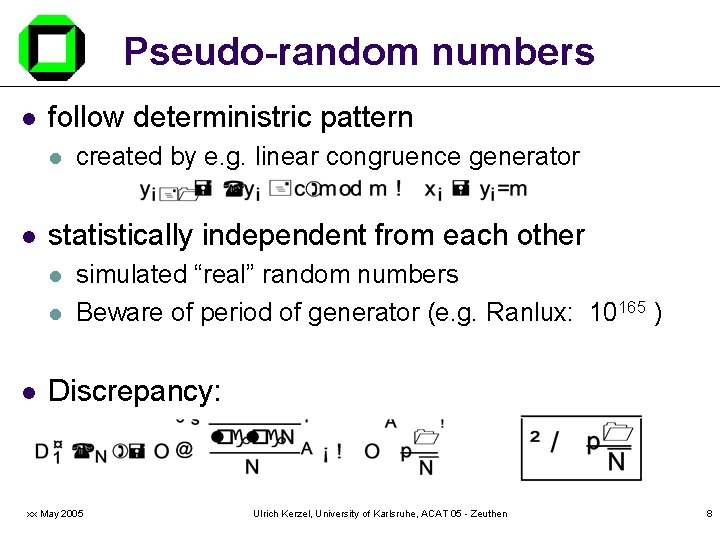
Pseudo-random numbers l follow deterministric pattern l l statistically independent from each other l l l created by e. g. linear congruence generator simulated “real” random numbers Beware of period of generator (e. g. Ranlux: 10165 ) Discrepancy: xx May 2005 Ulrich Kerzel, University of Karlsruhe, ACAT 05 - Zeuthen 8

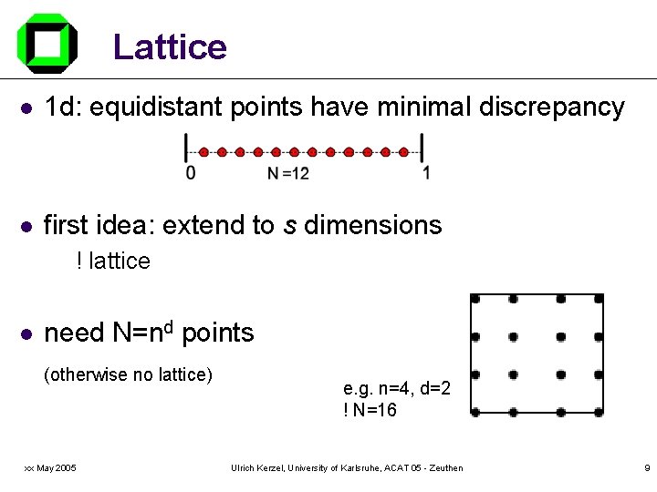
Lattice l 1 d: equidistant points have minimal discrepancy l first idea: extend to s dimensions ! lattice l need N=nd points (otherwise no lattice) xx May 2005 e. g. n=4, d=2 ! N=16 Ulrich Kerzel, University of Karlsruhe, ACAT 05 - Zeuthen 9

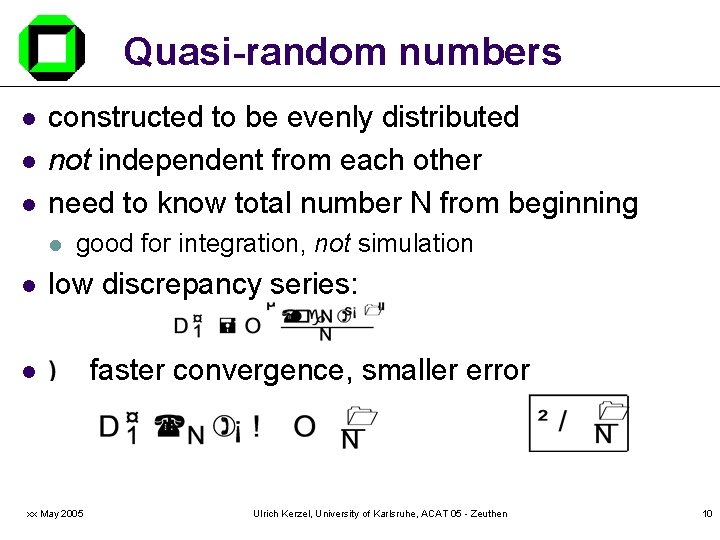
Quasi-random numbers l l l constructed to be evenly distributed not independent from each other need to know total number N from beginning l l good for integration, not simulation low discrepancy series: l xx May 2005 faster convergence, smaller error Ulrich Kerzel, University of Karlsruhe, ACAT 05 - Zeuthen 10

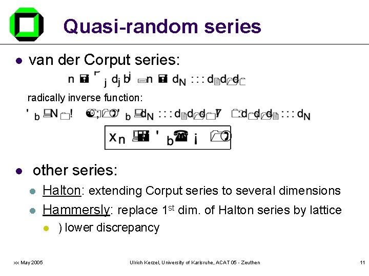
Quasi-random series l van der Corput series: radically inverse function: l other series: l l Halton: extending Corput series to several dimensions Hammersly: replace 1 st dim. of Halton series by lattice l xx May 2005 ) lower discrepancy Ulrich Kerzel, University of Karlsruhe, ACAT 05 - Zeuthen 11

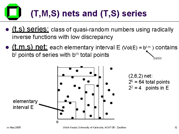
(T, M, S) nets and (T, S) series l (t, s) series: class of quasi-random numbers using radically inverse functions with low discrepancy l (t, m, s) net: each elementary interval E (Vol(E) = bt-m ) contains bt points of series with bm total points basis (2, 6, 2) net: 26 = 64 total points 22 = 4 points in E elementary interval E xx May 2005 Ulrich Kerzel, University of Karlsruhe, ACAT 05 - Zeuthen 12

Pseudo- vs. Quasi-random l generate 2048 numbers pseudo random quasi random xx May 2005 Ulrich Kerzel, University of Karlsruhe, ACAT 05 - Zeuthen 13

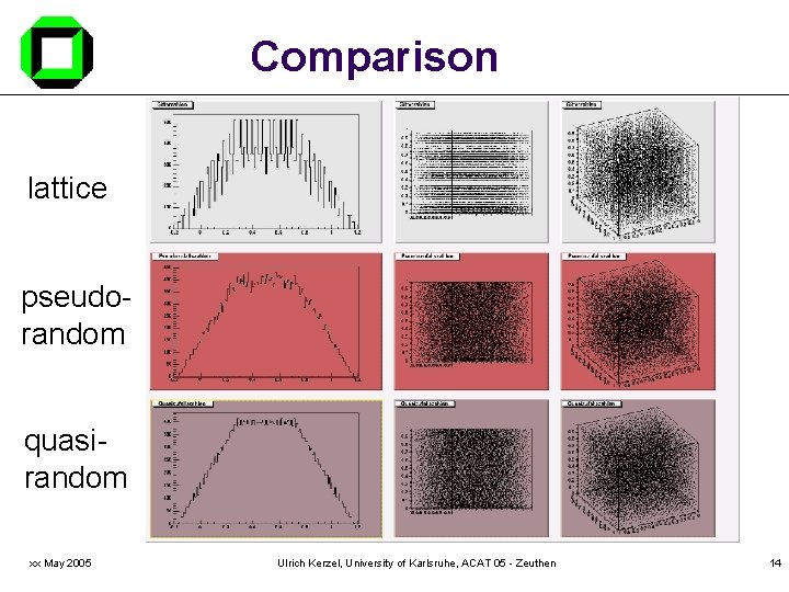
Comparison lattice pseudorandom quasirandom xx May 2005 Ulrich Kerzel, University of Karlsruhe, ACAT 05 - Zeuthen 14

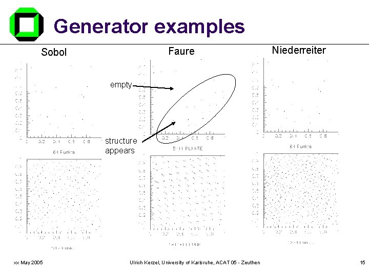
Generator examples Faure Sobol Niederreiter empty structure appears xx May 2005 Ulrich Kerzel, University of Karlsruhe, ACAT 05 - Zeuthen 15

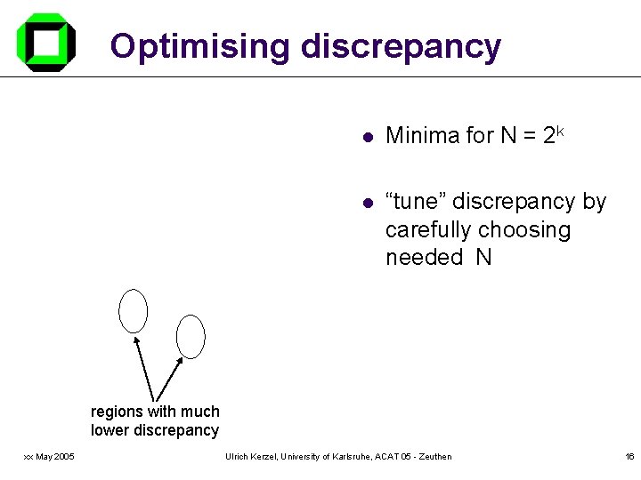
Optimising discrepancy l Minima for N = 2 k l “tune” discrepancy by carefully choosing needed N regions with much lower discrepancy xx May 2005 Ulrich Kerzel, University of Karlsruhe, ACAT 05 - Zeuthen 16

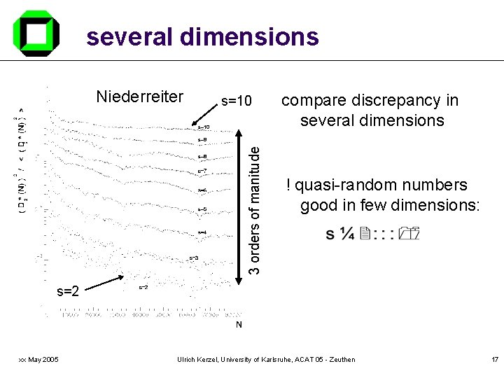
several dimensions s=10 3 orders of manitude Niederreiter compare discrepancy in several dimensions ! quasi-random numbers good in few dimensions: s=2 xx May 2005 Ulrich Kerzel, University of Karlsruhe, ACAT 05 - Zeuthen 17

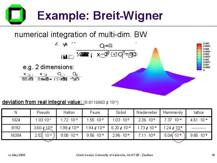
Example: Breit-Wigner numerical integration of multi-dim. BW e. g. 2 dimensions: deviation from real integral value: (8. 8116863 ¢ 10 -1) N Pseudo Halton Faure Sobol Niederreiter Hammersly lattice 1024 1. 03· 10 -1 1. 72 · 10 -2 1. 55 · 10 -2 1. 03 · 10 -2 2. 36 · 10 -3 7. 37 · 10 -4 4. 61 · 10 -4 8192 3. 60 ¢ 10 -2 1. 98 ¢ 10 -3 1. 94 ¢ 10 -3 6. 20 ¢ 10 -4 1. 73 ¢ 10 -4 1. 24 ¢ 10 -5 ------ 16384 2. 53 · 10 -2 9. 08 · 10 -4 9. 56 · 10 -4 2. 96 · 10 -4 7. 11 · 10 -5 5. 04 · 10 -6 9. 66 · 10 -5 xx May 2005 Ulrich Kerzel, University of Karlsruhe, ACAT 05 - Zeuthen 18

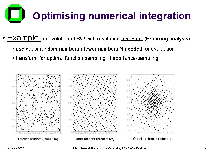
Optimising numerical integration • Example: convolution of BW with resolution per event (B 0 mixing analysis) • use quasi-random numbers ) fewer numbers N needed for evaluation • transform for optimal function sampling ) importance-sampling xx May 2005 Ulrich Kerzel, University of Karlsruhe, ACAT 05 - Zeuthen 19

Q-VEGAS l VEGAS: package for numerical integration in several dimensions: l l start with uniform intervals evaluate function values in these intervals iteratively adopt interval structure to shape of function Q-VEGAS: use quasi-random numbers instead of pseudo-random numbers: l faster and more accurate evaluation xx May 2005 Ulrich Kerzel, University of Karlsruhe, ACAT 05 - Zeuthen 20

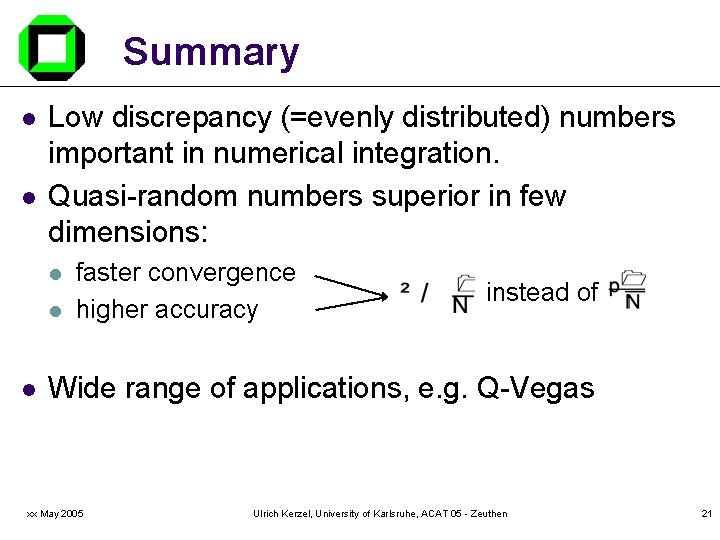
Summary l l Low discrepancy (=evenly distributed) numbers important in numerical integration. Quasi-random numbers superior in few dimensions: l l l faster convergence higher accuracy instead of Wide range of applications, e. g. Q-Vegas xx May 2005 Ulrich Kerzel, University of Karlsruhe, ACAT 05 - Zeuthen 21