
Fast Hierarchical Back Projection ECE 558 Final Project
Fast Hierarchical Back Projection ECE 558 Final Project Jason Chang Professor Kamalabadi May 8, 2007
Outline • Direct Filtered Back Projection (FBP) • Fast Hierarchical Back Projection (FHBP) • FHBP Results and Comparisons
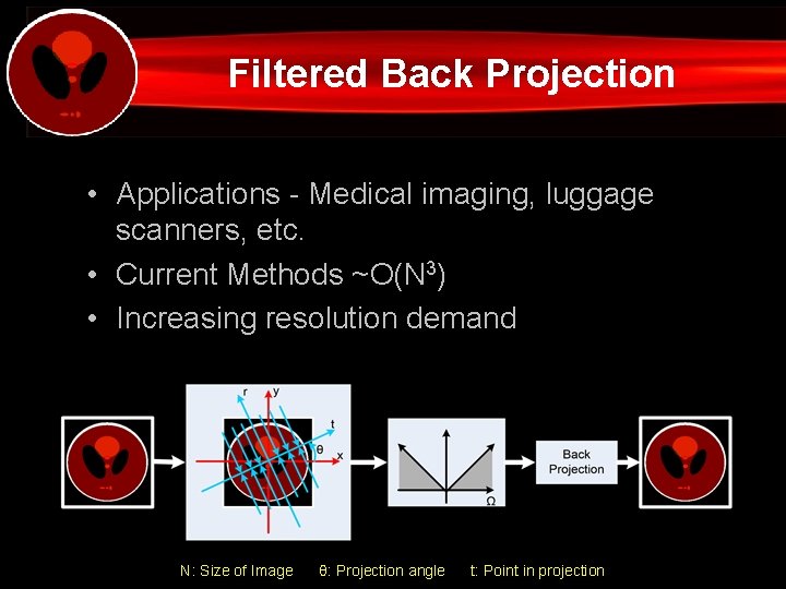
Filtered Back Projection • Applications - Medical imaging, luggage scanners, etc. • Current Methods ~O(N 3) • Increasing resolution demand N: Size of Image θ: Projection angle t: Point in projection
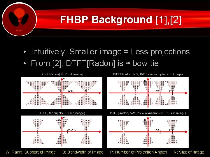
FHBP Background [1], [2] • Intuitively, Smaller image = Less projections • From [2], DTFT[Radon] is ≈ bow-tie W: Radial Support of Image B: Bandwidth of Image P: Number of Projection Angles N: Size of Image
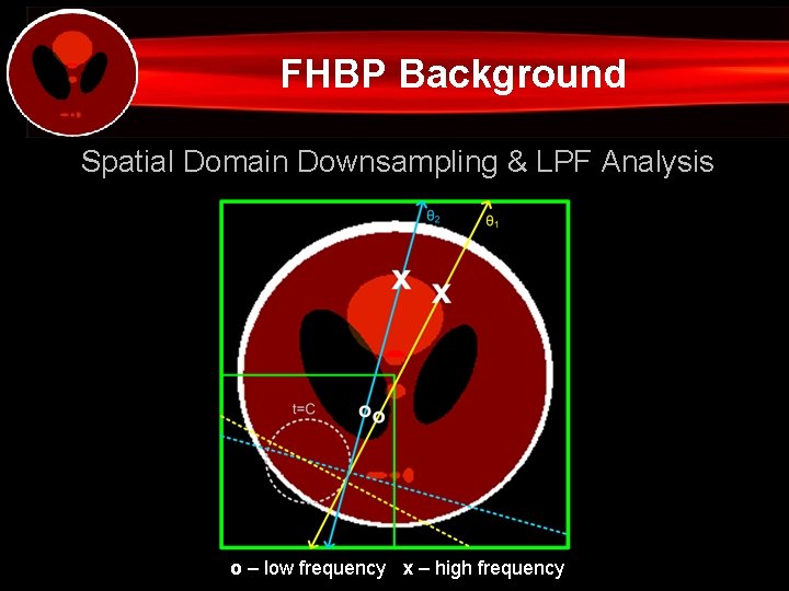
FHBP Background Spatial Domain Downsampling & LPF Analysis o – low frequency x – high frequency
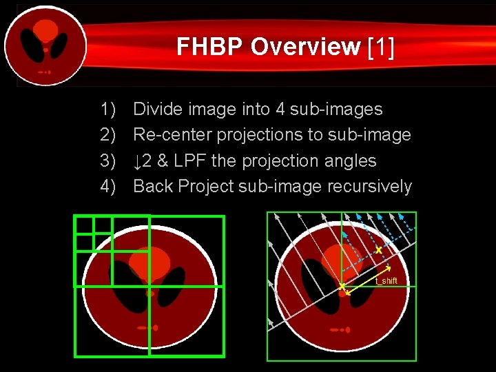
FHBP Overview [1] 1) 2) 3) 4) Divide image into 4 sub-images Re-center projections to sub-image ↓ 2 & LPF the projection angles Back Project sub-image recursively
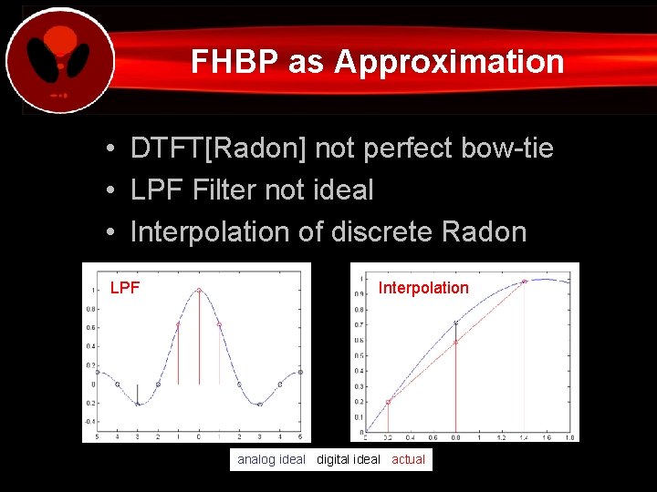
FHBP as Approximation • DTFT[Radon] not perfect bow-tie • LPF Filter not ideal • Interpolation of discrete Radon LPF Interpolation analog ideal digital ideal actual
Improving FHBP Parameters • Begin downsampling at level Q of recursion • Increase LPF length • Interpolate Np (radially) by M prior to backprojecting Notes [3]: • Q changes speed exponentially • M changes speed linearly Q: Number of non-downsampling levels Np: Number of points per projection M: Radial interpolation factor
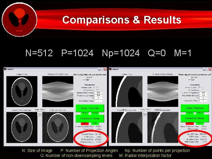
Comparisons & Results N=512 P=1024 Np=1024 Q=0 M=1 N: Size of Image P: Number of Projection Angles Np: Number of points per projection Q: Number of non-downsampling levels M: Radial interpolation factor
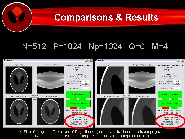
Comparisons & Results N=512 P=1024 Np=1024 Q=0 M=4 N: Size of Image P: Number of Projection Angles Np: Number of points per projection Q: Number of non-downsampling levels M: Radial interpolation factor
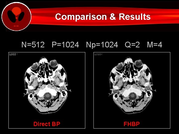
Comparison & Results N=512 P=1024 Np=1024 Q=2 M=4 Direct BP FHBP
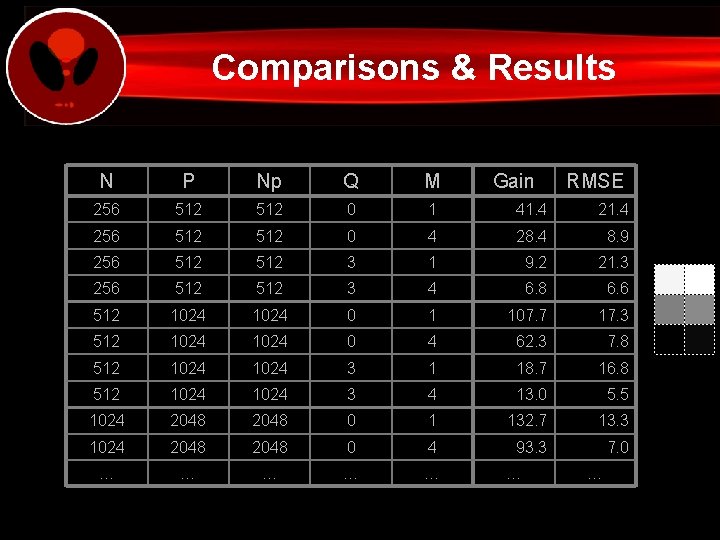
Comparisons & Results N P Np Q M Gain 256 512 0 1 41. 4 256 512 0 4 28. 4 8. 9 256 512 3 1 9. 2 21. 3 256 512 3 4 6. 8 6. 6 512 1024 0 1 107. 7 17. 3 512 1024 0 4 62. 3 7. 8 512 1024 3 1 18. 7 16. 8 512 1024 3 4 13. 0 5. 5 1024 2048 0 1 132. 7 13. 3 1024 2048 0 4 93. 3 7. 0 … … … RMSE …
Conclusions & Future Work • FHBP is much faster without much loss • Parameters allow for specific applications – LPF taps, Q, M • Implementation speed – Matlab vs. C++ vs. Assembly
References [1] S. Basu and Y. Bresler, “O(N 2 log 2 N) Filtered Backprojection Reconstruction Algorithm for Tomography, ” IEEE Trans. Image Processing, vol. 9, pp. 1760 -1773, October 2000. [2] P. A. Rattey and A. G. Lindgren, “Sampling the 2 -D Radon Transform, ” IEEE Trans. Acoustic, Speech, and Signal Processing, vol. ASSP-29, pp. 994 -1002, October, 1981. [3] S. Basu and Y. Bresler, “Error Analysis and Performance Optimization of Fast Hierarchical Backprojection Algorithms, ” IEEE Trans. Image Processing, vol. 10, pp. 1103 -1117, July 2001.

Thanks for coming! Questions?
- Slides: 15