Fast Convolution Chapter 8 Fast Convolution Introduction CookToom

Fast Convolution

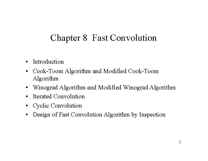
Chapter 8 Fast Convolution • Introduction • Cook-Toom Algorithm and Modified Cook-Toom Algorithm • Winograd Algorithm and Modified Winograd Algorithm • Iterated Convolution • Cyclic Convolution • Design of Fast Convolution Algorithm by Inspection 2

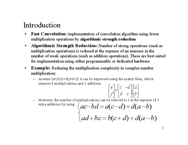
Introduction • Fast Convolution: implementation of convolution algorithm using fewer multiplication operations by algorithmic strength reduction • Algorithmic Strength Reduction: Number of strong operations (such as multiplication operations) is reduced at the expense of an increase in the number of weak operations (such as addition operations). These are best suited for implementation using either programmable or dedicated hardware • Example: Reducing the multiplication complexity in complex number multiplication: – Assume (a+jb)(c+dj)=e+jf, it can be expressed using the matrix form, which requires 4 multiplications and 2 additions: e c d a f d c b – However, the number of multiplications can be reduced to 3 at the expense of 3 extra additions by using: ac bd a(c d) d(a b) ad bc b(c d) d(a b) 3

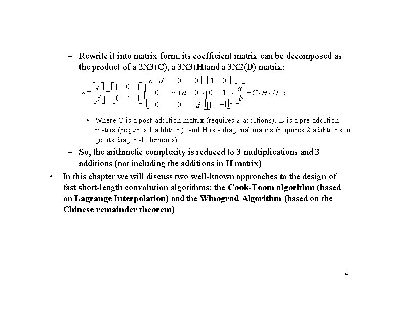
– Rewrite it into matrix form, its coefficient matrix can be decomposed as the product of a 2 X 3(C), a 3 X 3(H)and a 3 X 2(D) matrix: 0 c d e 1 0 1 s 0 c d f 0 1 1 0 0 0 1 0 a 0 0 1 C H D x b 1 d 1 • Where C is a post-addition matrix (requires 2 additions), D is a pre-addition matrix (requires 1 addition), and H is a diagonal matrix (requires 2 additions to get its diagonal elements) • – So, the arithmetic complexity is reduced to 3 multiplications and 3 additions (not including the additions in H matrix) In this chapter we will discuss two well-known approaches to the design of fast short-length convolution algorithms: the Cook-Toom algorithm (based on Lagrange Interpolation) and the Winograd Algorithm (based on the Chinese remainder theorem) 4

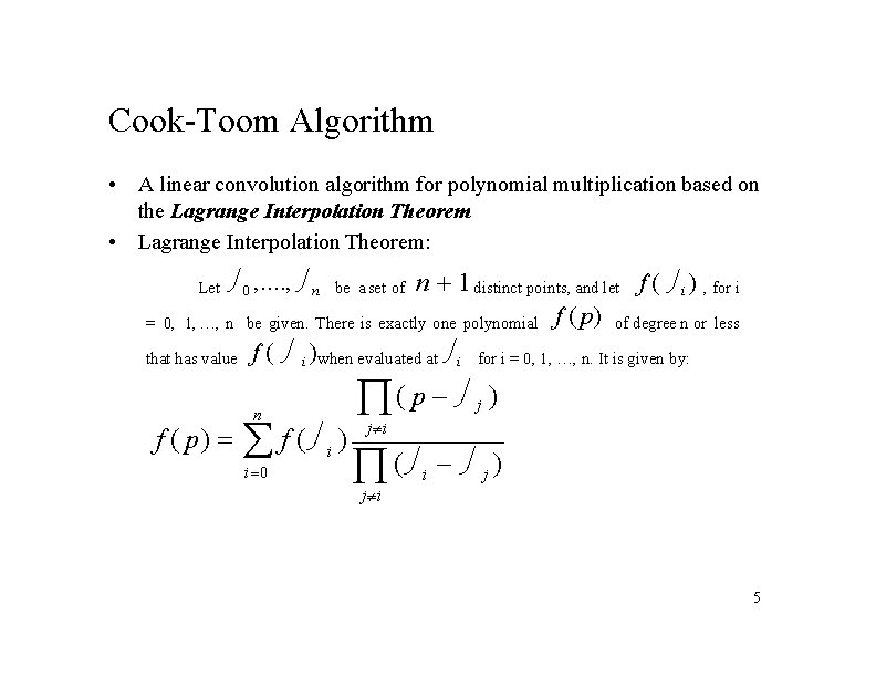
Cook-Toom Algorithm • A linear convolution algorithm for polynomial multiplication based on the Lagrange Interpolation Theorem • Lagrange Interpolation Theorem: Let 0 , . . , n be a set of n 1 distinct points, and let f ( i ) , for i = 0, 1, …, n be given. There is exactly one polynomial that has value f ( i )when evaluated at i n f ( p) f ( i ) i 0 ( p f ( p) of degree n or less for i = 0, 1, …, n. It is given by: j ) j i ( j i i j) 5

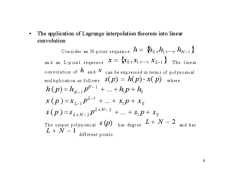
• The application of Lagrange interpolation theorem into linear convolution h h 0 , h 1 , . . . , h N 1 x x 0 , x 1 , . . . , x L 1 . The linear Consider an N-point sequence and an L-point sequence convolution of h and x can be expressed in terms of polynomial s ( p ) h ( p ) x( p) . . . h 1 p h 0 multiplication as follows: where h ( p ) h N 1 p. N 1 x ( p ) x L 1 p L 1 . . . x 1 p x 0 s ( p ) s L N 2 p L N 2 . . . s 1 p s 0 L N 2 The output polynomial s (p) has degree L N 1 different points. and has 6

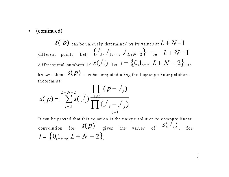
• (continued) L N 1 different points. Let 0 , 1 , . . . , L N 2 be L N 1 different real numbers. If s( i ) for i 0, 1, . . . , L N 2 are known, then s( p ) can be computed using the Lagrange interpolation s( p) theorem as: s( p) can be uniquely determined by its values at (p ) s( ) j L N 2 j i i i 0 i j j i It can be proved that this equation is the unique solution to compute linear convolution for s( p ) given i 0, 1, . . . , L N 2. the values of s( i ) , for 7

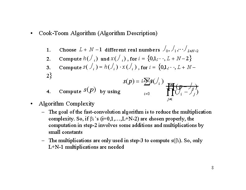
• Cook-Toom Algorithm (Algorithm Description) 1. 2. 3. 2 4. 0 , 1 , L N 2 Compute h( i ) and x( i ) , for i 0, 1, , L N 2 Compute s( i ) h( i ) x( i ) , for i 0, 1, , L N Choose L N 1 different real numbers Compute s ( p) • Algorithm Complexity N 2 s( p) L s( i ) by using i 0 (( p )) j i i j j j i – The goal of the fast-convolution algorithm is to reduce the multiplication complexity. So, if i `s (i=0, 1, …, L+N-2) are chosen properly, the computation in step-2 involves some additions and multiplications by small constants – The multiplications are only used in step-3 to compute s( i). So, only L+N-1 multiplications are needed 8

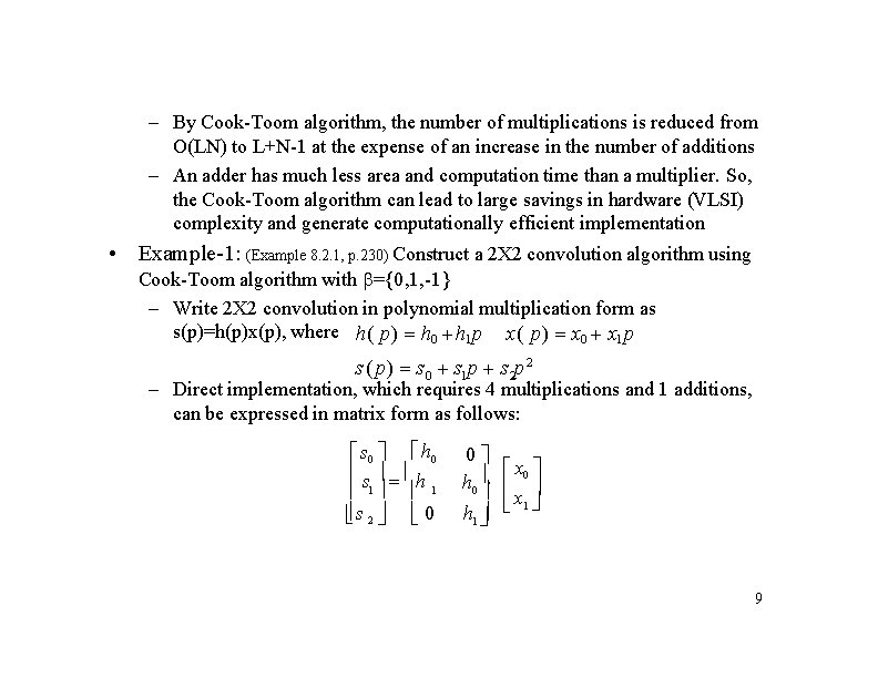
– By Cook-Toom algorithm, the number of multiplications is reduced from O(LN) to L+N-1 at the expense of an increase in the number of additions – An adder has much less area and computation time than a multiplier. So, the Cook-Toom algorithm can lead to large savings in hardware (VLSI) complexity and generate computationally efficient implementation • Example-1: (Example 8. 2. 1, p. 230) Construct a 2 X 2 convolution algorithm using Cook-Toom algorithm with ={0, 1, -1} – Write 2 X 2 convolution in polynomial multiplication form as s(p)=h(p)x(p), where h( p) h 0 h 1 p x( p) x 0 x 1 p s ( p) s 0 s 1 p s 2 p 2 – Direct implementation, which requires 4 multiplications and 1 additions, can be expressed in matrix form as follows: s 0 h 0 s h 1 1 s 2 0 0 x h 0 0 x h 1 1 9

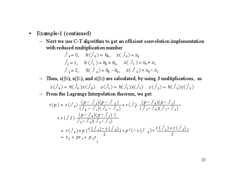
• Example-1 (continued) – Next we use C-T algorithm to get an efficient convolution implementation with reduced multiplication number 0 0, h ( 0 ) h 0 , x( 0 ) x 0 1 1, h ( 1 ) h 0 h 1 , x( 1 ) x 0 x 1 2 2, h( 2 ) h 0 h 1 , x( 2 ) x 0 x 1 – Then, s( 0), s( 1), and s( 2) are calculated, by using 3 multiplications, as s ( 0 ) h( 0 ) x ( 0 ) s ( 1 ) h( 1 ) x( 1 ) s ( 2 ) h( 2 ) x( 2 ) – From the Lagrange Interpolation theorem, we get: ( p 1 )( p 2 ) ( p 0 )( p 1 ) s ( 1) ( 0 1 )( 0 2 ) ( 1 0 )( 1 2 ) ( p 0 )( p 1 ) ( s( 2) 2 0 )( 2 1 ) s( p) s( 0) s ( 0 ) p ( s ( 1 ) s ( 2 ) ) p 2 ( s ( 2 s 0 ps 1 p 2 s 0 ) s ( 1) s ( 2) ) 2 2 10

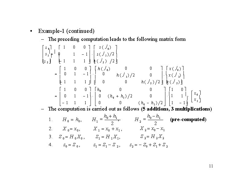
• Example-1 (continued) – The preceding computation leads to the following matrix form 1 0 0 1 0 1 s 0 s 1 s 2 1 1 1 0 s ( 0) 1 s ( 1 ) 2 1 s ( 2 ) 2 0 1 1 h ( 0) 0 0 0 1 1 h 0 0 0 x ( 0 ) h ( 1) 2 x ( 1) h ( 2 ) 2 x ( 2 ) 0 0 1 x 1 0 ( h 0 h 1 ) 2 1 0 x 0 ( h 0 h 1 ) 2 1 1 1 0 0 0 – The computation is carried out as follows (5 additions, 3 multiplications) h h 1. H 0 h 0 , H 1 0 1, (pre-computed) H 2 0 1 2 2 X 2 x 0 x 1 2. X 0 x 0 , X 1 x 0 x 1 , S 2 H 2 X 2 3. S 0 H 0 X 0 , S 1 H 1 X 1 , 4. s 0 S 0 , s 1 S 2 , s 2 S 0 S 1 S 2 11

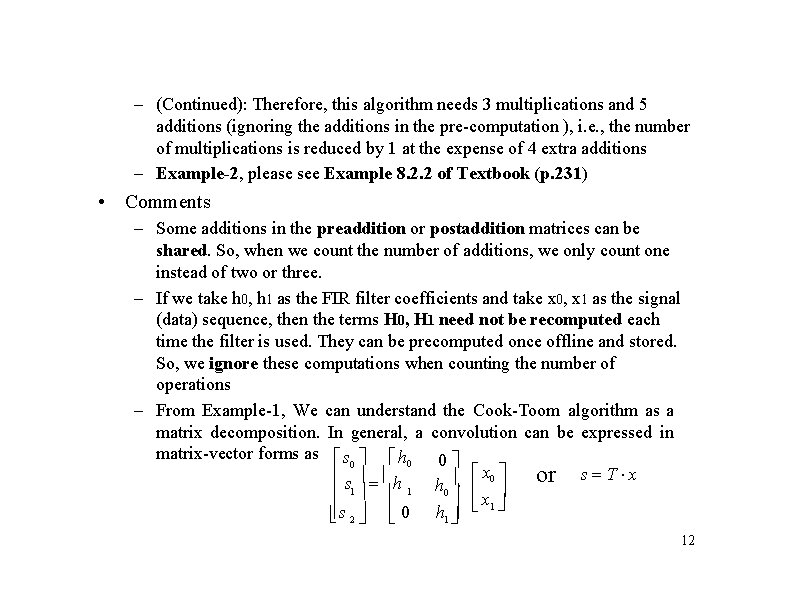
– (Continued): Therefore, this algorithm needs 3 multiplications and 5 additions (ignoring the additions in the pre-computation ), i. e. , the number of multiplications is reduced by 1 at the expense of 4 extra additions – Example-2, please see Example 8. 2. 2 of Textbook (p. 231) • Comments – Some additions in the preaddition or postaddition matrices can be shared. So, when we count the number of additions, we only count one instead of two or three. – If we take h 0, h 1 as the FIR filter coefficients and take x 0, x 1 as the signal (data) sequence, then the terms H 0, H 1 need not be recomputed each time the filter is used. They can be precomputed once offline and stored. So, we ignore these computations when counting the number of operations – From Example-1, We can understand the Cook-Toom algorithm as a matrix decomposition. In general, a convolution can be expressed in matrix-vector forms as s 0 h 0 0 or s T x s h x 0 h 1 1 0 x 1 s 2 0 h 1 12

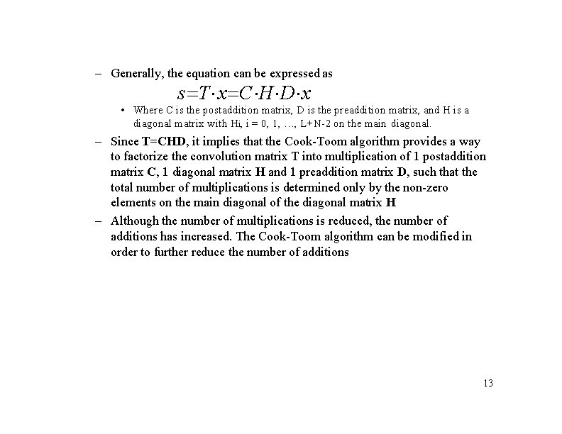
– Generally, the equation can be expressed as s T x C H D x • Where C is the postaddition matrix, D is the preaddition matrix, and H is a diagonal matrix with Hi, i = 0, 1, …, L+N-2 on the main diagonal. – Since T=CHD, it implies that the Cook-Toom algorithm provides a way to factorize the convolution matrix T into multiplication of 1 postaddition matrix C, 1 diagonal matrix H and 1 preaddition matrix D, such that the total number of multiplications is determined only by the non-zero elements on the main diagonal of the diagonal matrix H – Although the number of multiplications is reduced, the number of additions has increased. The Cook-Toom algorithm can be modified in order to further reduce the number of additions 13

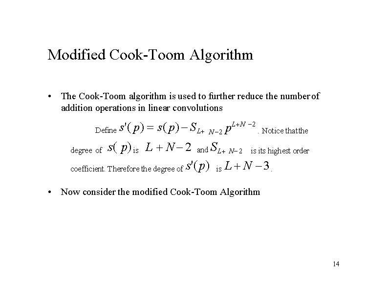
Modified Cook-Toom Algorithm • The Cook-Toom algorithm is used to further reduce the number of addition operations in linear convolutions Define s'( p) s( p) SL L N 2 p. Notice that the N 2 s( p) is L N 2 and S L N 2 is its highest order coefficient. Therefore the degree of s'( p) is L N 3. degree of • Now consider the modified Cook-Toom Algorithm 14

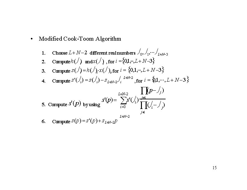
• Modified Cook-Toom Algorithm 1. 2. Choose L N 2 different real numbers 0 , 1, L N 3 Compute h( i) and x( )i , for i 0, 1, , L N 3 3. Compute s( i) h( )i x( )i, for i 0, 1, , L N 3 4. Compute s'( i ) s. L N 2 i 5. Compute s'(p) by using s'(p) L N 2 , for i 0, 1, , L N 3 L N 2 (p ) i 0 ( ) s'( i) j j i i j j i 6. Compute s( p) s'( p) s. L N 2 p L N 2 15

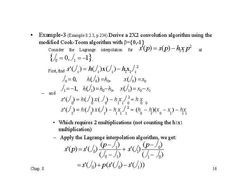
• Example-3 (Example 8. 2. 3, p. 234) Derive a 2 X 2 convolution algorithm using the modified Cook-Toom algorithm with ={0, -1} Consider the Lagrange 0 0, 1 1. First, find – and interpolation for s'( p) s( p) h 1 x 1 p 2 at s'( i ) h( i )x( i ) h 1 x 1 i 2 0 0, h( 0) h 0, 1 1, h( 1) h 0 h 1, x( 0) x 0 x( 1) x 0 x 1 s'( ) h( ) x( ) h x 2 h x 0 0 0 1 1 0 2 0 0 s'( ) h( ) x( ) h x (h h )( x x ) h x 1 1 1 0 1 11 • Which requires 2 multiplications (not counting the h 1 x 1 multiplication) – Apply the Lagrange interpolation algorithm, we get: ( p 1) ( p 0) s'( p) s'( 0) s'( 1) ( 0 1) ( 1 0) Chap. 8 s'( 0 ) p(s'( 0) s'( 1)) 16

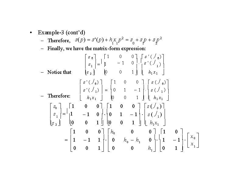
• Example-3 (cont’d) 2 2 – Therefore, s( p) s' ( p) h 1 x 1 p s 0 s 1 p s 2 p – Finally, we have the matrix-form expression: – Notice that – Therefore: s 0 1 s 1 1 0 s 2 1 1 0 1 s 0 s 1 1 0 s 2 0 1 0 1 s ' ( 0) s ' ( ) 0 1 0 h 1 x 1 0 0 1 0 0 1 0 0 h 0 1 0 0 s ' ( 0 ) 0 s ' ( ) 1 1 h 1 x 1 0 s ( 0 ) 1 s ( 1 ) 1 h 1 x 1 0 0 s ( 0 ) 1 s ( 1 ) 1 h 1 x 1 0 h 0 h 1 0 0 1 0 1 h 1 0 0 x 1 0 x 1 1

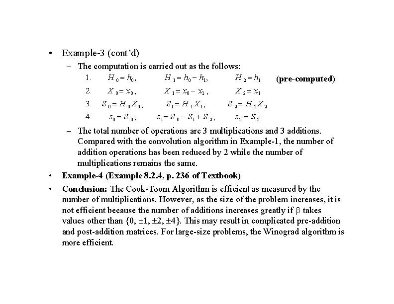
• Example-3 (cont’d) – The computation is carried out as the follows: 1. H 0 h 0, H 1 h 0 h 1, H 2 h 1 2. X 0 x 0 , X 1 x 0 x 1 , X 2 x 1 3. S 0 H 0 X 0 , S 1 H 1 X 1 , S 2 H 2 X 2 4. s 0 S 0 , s 1 S 0 S 1 S 2 , s 2 S 2 • • (pre-computed) – The total number of operations are 3 multiplications and 3 additions. Compared with the convolution algorithm in Example-1, the number of addition operations has been reduced by 2 while the number of multiplications remains the same. Example-4 (Example 8. 2. 4, p. 236 of Textbook) Conclusion: The Cook-Toom Algorithm is efficient as measured by the number of multiplications. However, as the size of the problem increases, it is not efficient because the number of additions increases greatly if takes values other than {0, 1, 2, 4}. This may result in complicated pre-addition and post-addition matrices. For large-size problems, the Winograd algorithm is more efficient.

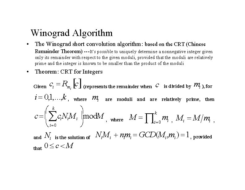
Winograd Algorithm • The Winograd short convolution algorithm: based on the CRT (Chinese Remainder Theorem) ---It’s possible to uniquely determine a nonnegative integer given only its remainder with respect to the given moduli, provided that the moduli are relatively prime and the integer is known to be smaller than the product of the moduli • Theorem: CRT for Integers ci Rmi c (represents the remainder when c i 0, 1, . . . , k , where mi are moduli and are Given is divided by mi ), for relatively prime, then k c ci. Ni M i mod. M , where M k mi , Mi M mi , i 0 and Ni is the solution of Ni Mi nimi GCD(Mi, mi ) 1 , provided that 0 c M

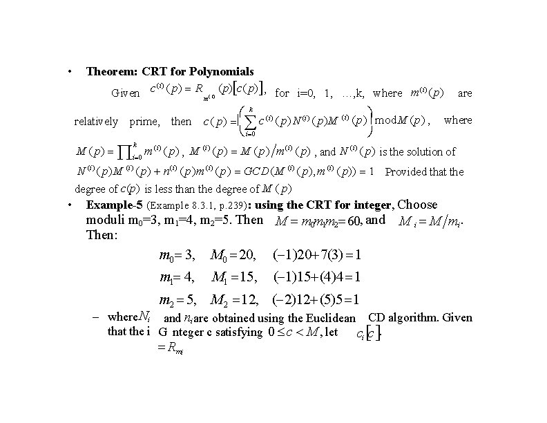
• Theorem: CRT for Polynomials (i ) Given c ( p) R m ( p) c( p) , for i=0, 1, …, k, where m( i) ( p) ( i) are k (i) relatively prime, then c( p) c ( p) N (i) ( p)M ( i) ( p) mod M ( p) , where i 0 k M ( p) i 0 m (i) ( p) , M (i) ( p) M ( p) m(i ) ( p) , and N (i) ( p) is the solution of N (i) ( p)M (i) ( p) n(i ) ( p)m (i) ( p) GCD (M (i) ( p), m (i) ( p)) 1 Provided that the degree of c(p) is less than the degree of M ( p) • Example-5 (Example 8. 3. 1, p. 239): using the CRT for integer, Choose moduli m 0=3, m 1=4, m 2=5. Then M m 0 m 1 m 2 60, and Then: m 0 3, m 1 4, M 0 20, M 1 15, M i M mi. ( 1)20 7(3) 1 ( 1)15 (4)4 1 m 2 5, M 2 12, ( 2)12 (5)5 1 – where Ni and ni are obtained using the Euclidean CD algorithm. Given that the i G nteger c satisfying 0 c M , let ci c . Rmi

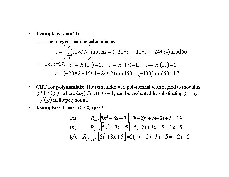
• Example-5 (cont’d) – The integer c can be calculated as k c ci. Ni. M i mod. M ( 20 c 0 15 c 1 24 c 2) mod 60 i 0 – For c=17, c 0 R 3(17) 2, c 1 R 4(17) 1, c 2 R 5(17) 2 c ( 20 2 15 1 24 2) mod 60 103 mod 60 17 • • CRT for polynomials: The remainder of a polynomial with regard to modulus pi f ( p) , where deg( f ( p)) i 1, can be evaluated by substituting pi by f ( p) in the polynomial Example-6 (Example 8. 3. 2, pp 239) (a). (b). R 5 x 3 x 5 5( 2) 3 x 5 5 x 3 x 5 5( x 2) 3 x 5 2 x 5 Rx 2 5 x 2 3 x 5 5( 2)2 3( 2) 5 19 2 2 x 2 (c). Rx 2 2

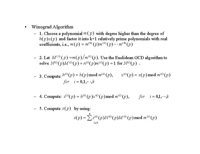
• Winograd Algorithm – 1. Choose a polynomial m( p) with degree higher than the degree of h( p) x( p) and factor it into k+1 relatively prime polynomials with real coefficients, i. e. , m( p) m ( 0) ( p)m (1) ( p) m ( k ) ( p) – 2. Let M ( i) ( p) m( p) m ( i) ( p). Use the Euclidean GCD algorithm to solve N (i ) ( p)M (i ) ( p) n( i ) ( p)m ( i ) ( p) 1 for N (i ) ( p). (i ) ( i) – 3. Compute: h ( p) h( p) mod m ( p), for i 0, 1, , k x( i ) ( p) x( p) mod m ( i) ( p) – 4. Compute: s ( i ) ( p) h( i) ( p)x (i) ( p) mod m ( i) ( p), for i 0, 1, , k – 5. Compute s( p) by using: k s( p) s ( i) ( p)N (i ) ( p)M (i) ( p) mod m ( i) ( p) i 0

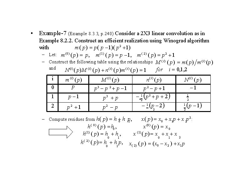
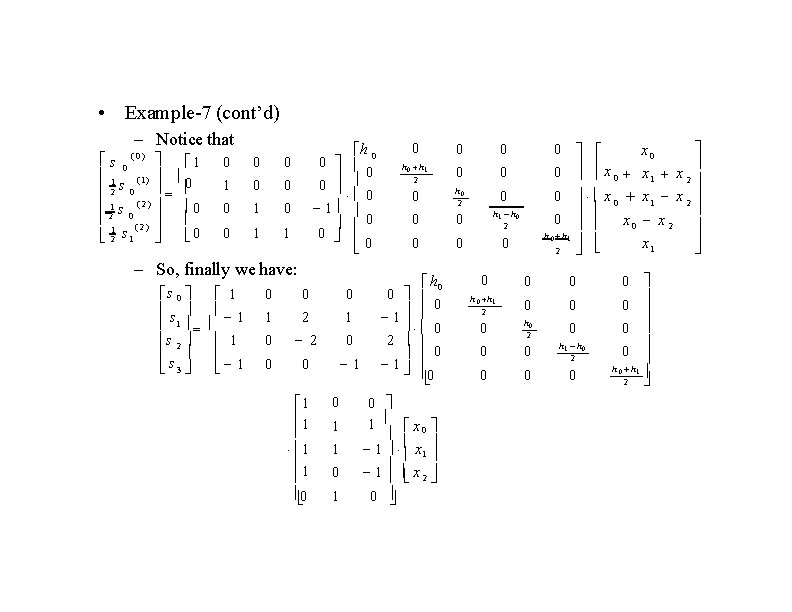
• Example-7 (Example 8. 3. 3, p. 240) Consider a 2 X 3 linear convolution as in Example 8. 2. 2. Construct an efficient realization using Winograd algorithm with m( p) p( p 1)( p 2 1) – Let: m ( 0) ( p) p, m(1) ( p) p 1, m ( 2) ( p) p 2 1 – Construct the following table using the relationships M ( i) ( p) m( p) m ( i) ( p) and for i 0, 1, 2 N (i ) ( p)M (i) ( p) n ( i) ( p)m ( i) ( p) 1 i 0 m (i) ( p) p M (i ) ( p) p 3 p 2 p 1 1 p 3 p n(i ) ( p) p 2 p 1 1 p 2 p 2 2 p 2 1 p 2 0 1 1 2 2 1 p 2 – Compute residues from h( p) h 0 h p, 1 h ( 0) ( p) h 0 , h(1) ( p) h h , 0 1 ( 2) h ( p) h h p, N (i) ( p) 1 1 2 p 1 x( p) x 0 x 1 p x 2 p 2 : x (0) ( p) x 0 x (1) ( p) x x x 2 0 1 x( 2) ( p) (x 0 x 2 ) x 1 p

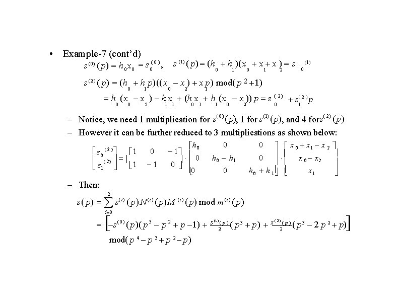
• Example-7 (cont’d) s (1) ( p) (h h )( x x x ) s (0) ( p) h 0 x 0 s 0 , 0 1 2 (1) 0 s (2) ( p) (h h p)(( x x ) x p) mod( p 2 1) 0 1 0 2 1 h ( x x ) h x (h x h (x x )) p s ( 2) s( 2 ) p 0 0 2 1 1 0 2 0 1 – Notice, we need 1 multiplication for s ( 0 ) ( p), 1 for s (1) ( p), and 4 fors ( 2) ( p) – However it can be further reduced to 3 multiplications as shown below: s 0 ( 2 ) 1 ( 2) s 1 1 0 1 h 0 1 0 0 x 0 x 1 x 2 0 x 2 h 0 h 1 x 1 0 h 0 h 1 0 – Then: 2 s( p) s ( i) ( p) N (i ) ( p)M (i ) ( p) mod m (i ) ( p) i 0 s ( 0 ) ( p)( p 3 p 2 p 1) S mod( p 4 p 3 p 2 p) (1 ) (p) 2 ( p 3 p) S (2) (p) 2 ( p 3 2 p 2 p)

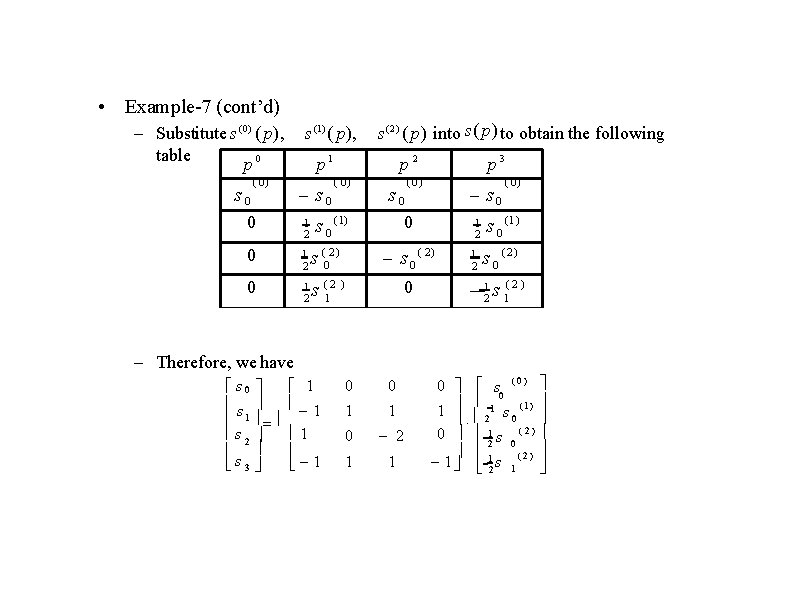
• Example-7 (cont’d) – Substitute s (0) ( p), table p 0 (0) s 0 0 s (1) ( p), s ( 2 ) ( p) into s( p) to obtain the following p 1 s 0 1 2 p 2 ( 0) s 0 (1) p 3 (0) s 0 0 1 2 s (02 ) s 0 ( 2) 0 1 2 s (12 ) 0 1 2 (0) s 0 (1 ) s 0 (2) 21 s 1( 2 ) – Therefore, we have s 0 1 1 s 1 s 2 1 s 3 1 0 0 1 1 0 2 1 1 0 s 0 ( 0 ) 1 21 s 0 ( 1 ) 0 12 s 0 ( 2 ) 1 12 s 1 ( 2 )

• Example-7 (cont’d) – Notice that s 0 1 1 (1 ) 2 s 0 0 1 s ( 2) 0 2 0( 2) 1 0 2 s 1 ( 0) 0 0 0 1 1 h 0 0 0 1 0 0 0 – So, finally we have: s 0 s 1 s 2 s 3 1 1 0 2 0 1 1 1 0 2 0 0 0 1 1 1 0 0 1 1 0 h 0 h 1 2 0 0 0 h 0 2 0 0 0 h 1 h 0 2 0 0 0 h 0 0 0 1 0 2 0 1 0 0 1 x 0 1 x 1 1 x 2 0 0 0 x 0 0 x 0 h 0 h 1 2 0 0 h 0 2 0 0 h 1 h 0 2 0 0 0 x 1 x 2 x 1 x 0 0 0 h 1 2

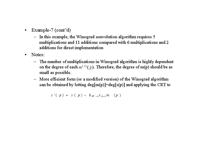
• Example-7 (cont’d) – In this example, the Winograd convolution algorithm requires 5 multiplications and 11 additions compared with 6 multiplications and 2 additions for direct implementation • Notes: – The number of multiplications in Winograd algorithm is highly dependent on the degree of each m ( i ) ( p). Therefore, the degree of m(p) should be as small as possible. – More efficient form (or a modified version) of the Winograd algorithm can be obtained by letting deg[m(p)]=deg[s(p)] and applying the CRT to s '( p ) s ( p) h N 1 x L 1 m (p )

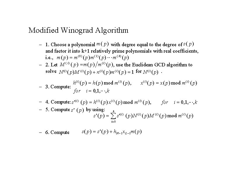
Modified Winograd Algorithm – 1. Choose a polynomial m( p) with degree equal to the degree of s( p) and factor it into k+1 relatively prime polynomials with real coefficients, i. e. , m( p) m ( 0) ( p)m (1) ( p) m ( k ) ( p) – 2. Let M ( i) ( p) m( p) m ( i) ( p) , use the Euclidean GCD algorithm to solve N (i ) ( p)M (i ) ( p) n( i ) ( p)m ( i ) ( p) 1 for N (i ) ( p). – 3. Compute: h( i ) ( p) h( p) mod m ( i) ( p), for x( i ) ( p) x( p) mod m ( i) ( p) i 0, 1, , k – 4. Compute: s' ( i) ( p) h ( i) ( p) x( i ) ( p) mod m ( i) ( p), for i 0, 1, , k – 5. Compute s' ( p) by using: k s' ( p) s' ( i) ( p)N (i) ( p)M (i ) ( p) mod m ( i ) ( p) i 0 – 6. Compute s( p) s' ( p) h. N 1 x. L 1 m( p)

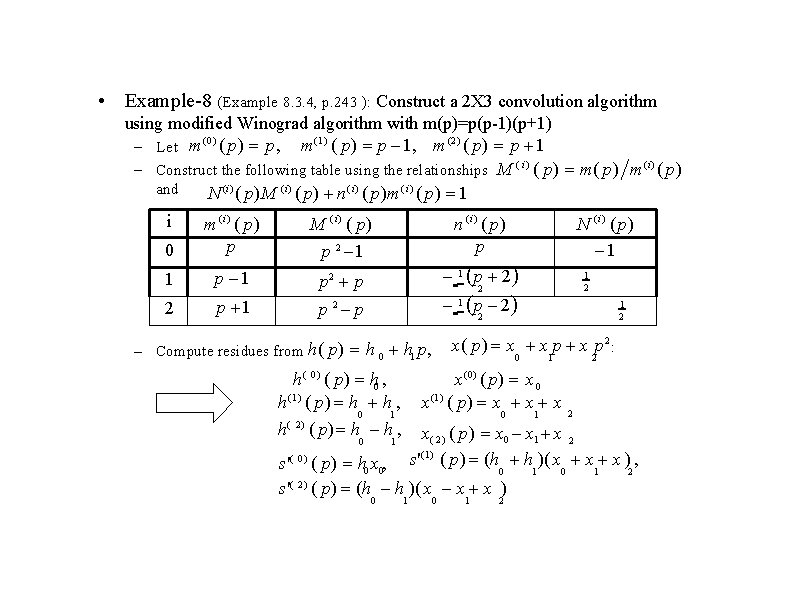
• Example-8 (Example 8. 3. 4, p. 243 ): Construct a 2 X 3 convolution algorithm using modified Winograd algorithm with m(p)=p(p-1)(p+1) (0) (1) (2) – Let m ( p) p, m ( p) p 1 – Construct the following table using the relationships M ( i) ( p) m( p) m ( i) ( p) and N (i ) ( p)M (i) ( p) n ( i) ( p)m ( i) ( p) 1 i M (i) ( p) 0 m (i) ( p) p 1 p 2 p n (i ) ( p) p p 2 1 N (i) ( p) 1 1 p 2 1 2 2 x( p) x x p 2 : 0 1 2 – Compute residues from h( p) h 0 h 1 p, h ( 0) ( p) h 0 , h(1) ( p) h h , 0 1 ( 2) h ( p) h h , 0 x (0) ( p) x 0 x(1) ( p) x x x 0 2 x( 2) ( p) x 0 x 1 x 2 s'(1) ( p) (h h )( x x x ) , 1 s' ( 0) ( p) h 0 x 0, 0 s' ( 2) ( p) (h h )( x x x ) 0 1 1 0 1 2

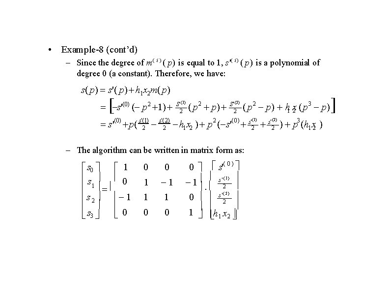
• Example-8 (cont’d) – Since the degree of m ( i ) ( p) is equal to 1, s' ( i) ( p) is a polynomial of degree 0 (a constant). Therefore, we have: s( p) s'( p) h 1 x 2 m( p) s'(0) ( p 2 1) S ' (1) 2 ( p 2 p) S ' ( 2) 2 ( p 2 p) h 1 x 2 ( p 3 p) s'(2) 2 (0) s' 3 s' s'(0) p( s'(1) h x ) p ( s' ) p (h 1 x 2 ) 1 2 2 2 (1) – The algorithm can be written in matrix form as: s 0 1 s 0 1 s 2 1 0 s 3 0 0 1 1 0 0 s'( 0 ) (1) 1 s '2 ( 2) 0 s '2 1 h 1 x 2 ( 2)

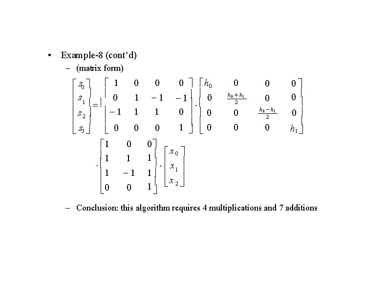
• Example-8 (cont’d) – (matrix form) 0 1 s 0 1 1 s 2 1 1 0 0 s 3 0 1 1 1 0 0 0 1 1 0 0 h 0 1 0 0 0 1 0 0 h 0 h 1 2 0 0 0 0 h 1 0 x 0 1 x 1 1 x 2 1 – Conclusion: this algorithm requires 4 multiplications and 7 additions

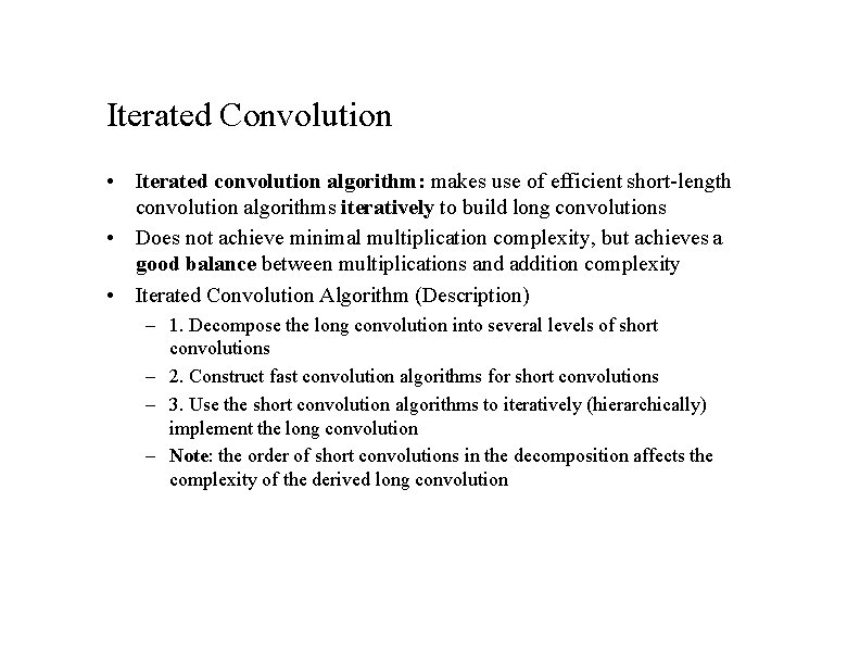
Iterated Convolution • Iterated convolution algorithm: makes use of efficient short-length convolution algorithms iteratively to build long convolutions • Does not achieve minimal multiplication complexity, but achieves a good balance between multiplications and addition complexity • Iterated Convolution Algorithm (Description) – 1. Decompose the long convolution into several levels of short convolutions – 2. Construct fast convolution algorithms for short convolutions – 3. Use the short convolution algorithms to iteratively (hierarchically) implement the long convolution – Note: the order of short convolutions in the decomposition affects the complexity of the derived long convolution

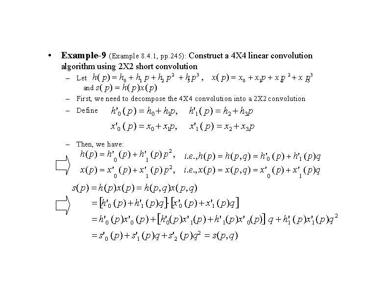
• Example-9 (Example 8. 4. 1, pp. 245): Construct a 4 X 4 linear convolution algorithm using 2 X 2 short convolution 2 3 2 x p 3 3 – Let h( p) h 0 h 1 p h 2 p h 3 p , x( p) x 0 x 1 p x p 2 and s( p) h( p)x( p) – First, we need to decompose the 4 X 4 convolution into a 2 X 2 convolution – Define h'0 ( p) h 0 h 1 p, h'1 ( p) h 2 h 3 p x'0 ( p) x 0 x 1 p, x'1 ( p) x 2 x 3 p – Then, we have: h( p) h' ( p) p 2 , i. e. , h( p) h( p, q) h'0 ( p) h'1 ( p)q 0 1 x( p) x' ( p) p 2 , i. e. , x( p) x( p, q) x' ( p)q 0 1 s( p) h( p)x( p) h( p, q)x( p, q) h'0 ( p) h'1 ( p)q x'0 ( p) x'1 ( p)q h'0 ( p)x' 0 ( p) h'0( p)x' 1( p) h' 1( p)x' 0( p) q h'1 ( p)x'1 ( p)q 2 s'0 ( p) s'1 ( p)q s' 2 ( p)q 2 s( p, q)

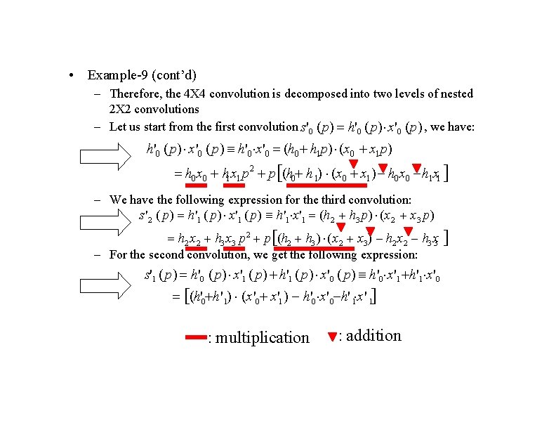
• Example-9 (cont’d) – Therefore, the 4 X 4 convolution is decomposed into two levels of nested 2 X 2 convolutions – Let us start from the first convolution s'0 ( p) h'0 ( p) x'0 ( p) , we have: h'0 ( p) x'0 ( p) h'0 x'0 (h 0 h 1 p) (x 0 x 1 p) h 0 x 0 h 1 x 1 p 2 p (h 0 h 1) (x 0 x 1 ) h 0 x 0 h 1 x 1 – We have the following expression for the third convolution: s'2 ( p) h'1 ( p) x'1 ( p) h'1 x'1 (h 2 h 3 p) (x 2 x 3 p) h 2 x 2 h 3 x 3 p 2 p (h 2 h 3 ) (x 2 x 3) h 2 x 2 h 3 x 3 – For the second convolution, we get the following expression: s'1 ( p) h'0 ( p) x'1 ( p) h'1 ( p) x'0 ( p) h'0 x'1 h'1 x'0 (h'0 h' 1) (x'0 x'1 ) h'0 x' 0 h' 1 x' 1 : multiplication : addition

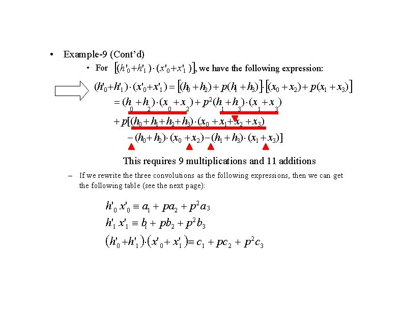
• Example-9 (Cont’d) • For (h'0 h'1 ) (x'0 x'1 ) , we have the following expression: (h'0 h'1 ) (x'0 x'1 ) (h 0 h 2 ) p(h 1 h 3) (x 0 x 2) p(x 1 x 3) (h h ) (x x ) p 2 (h h ) (x x ) 0 2 1 3 p[(h 0 h 1 h 2 h 3) (x 0 x 1 x 2 x 3) (h 0 h 2) (x 0 x 2 ) (h 1 h 3) (x 1 x 3)] This requires 9 multiplications and 11 additions – If we rewrite three convolutions as the following expressions, then we can get the following table (see the next page): h' 0 x'0 a 1 pa 2 p 2 a 3 h'1 x'1 b 1 pb 2 p 2 b 3 h'0 h'1 x' 0 x'1 c 1 pc 2 p 2 c 3

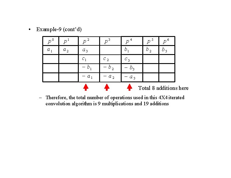
• Example-9 (cont’d) p 0 a 1 p 1 a 2 p 2 a 3 p 4 b 1 c 2 c 3 b 1 b 2 b 3 a 1 a 2 a 3 p 5 b 2 p 6 b 3 Total 8 additions here – Therefore, the total number of operations used in this 4 X 4 iterated convolution algorithm is 9 multiplications and 19 additions

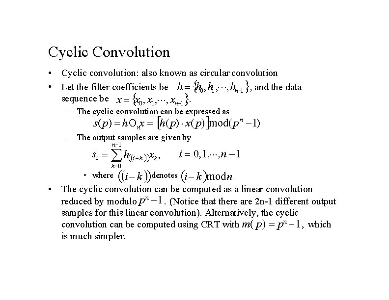
Cyclic Convolution • Cyclic convolution: also known as circular convolution • Let the filter coefficients be h h 0 , h 1 , , hn 1 , and the data sequence be x x 0 , x 1, , xn 1. – The cyclic convolution can be expressed as s( p) h nx h( p) x( p) mod( p n 1) – The output samples are given by n 1 si h i k xk , i 0, 1, , n 1 k 0 • where i k denotes i k mod n • The cyclic convolution can be computed as a linear convolution reduced by modulo p n 1. (Notice that there are 2 n-1 different output samples for this linear convolution). Alternatively, the cyclic convolution can be computed using CRT with m( p) pn 1 , which is much simpler.

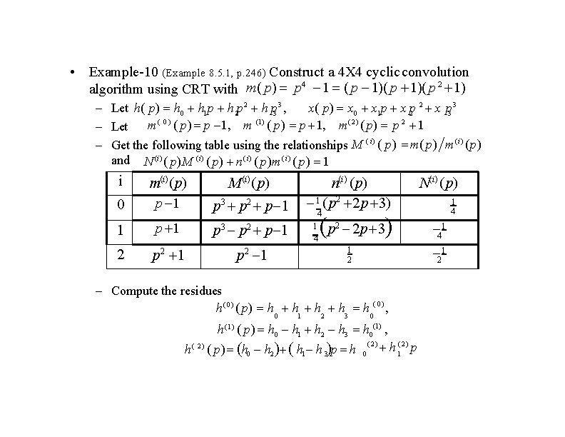
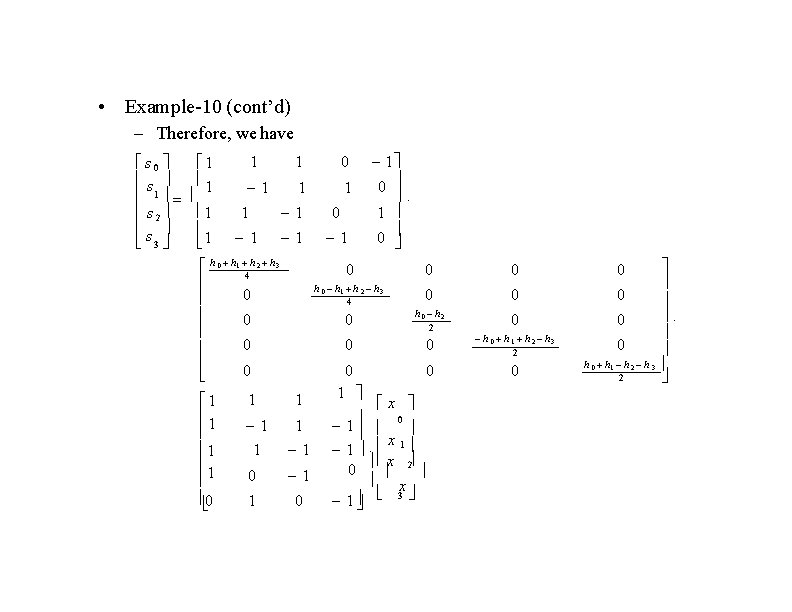
• Example-10 (Example 8. 5. 1, p. 246) Construct a 4 X 4 cyclic convolution algorithm using CRT with m( p) p 4 1 ( p 1)( p 2 1) – Let h( p) h 0 h 1 p h 2 p 2 h p 3 3 , x( p) x 0 x 1 p x p 2 2 x p 3 3 – Let m ( 0 ) ( p) p 1, m (1) ( p) p 1, m ( 2 ) ( p) p 2 1 – Get the following table using the relationships M ( i) ( p) m( p) m ( i) ( p) and N (i ) ( p)M (i) ( p) n ( i) ( p)m ( i) ( p) 1 i 0 m(i) ( p) p 1 M (i) ( p) p 3 p 2 p 1 1 p 3 p 2 p 1 2 p 2 1 n(i) ( p) 1 ( p 2 2 p 3) 4 1 4 p 2 p 3 2 – Compute the residues h ( 0 ) ( p) h h h ( 0) , 1 2 3 0 (1) 0 (2 ) h(1) ( p) h 0 h 1 h 2 h 3 h h ( 2) ( p) h 0 h 2 h 1 h 3 p h 1 4 41 21 1 2 0 N(i) ( p) 0 , h 1( 2) p

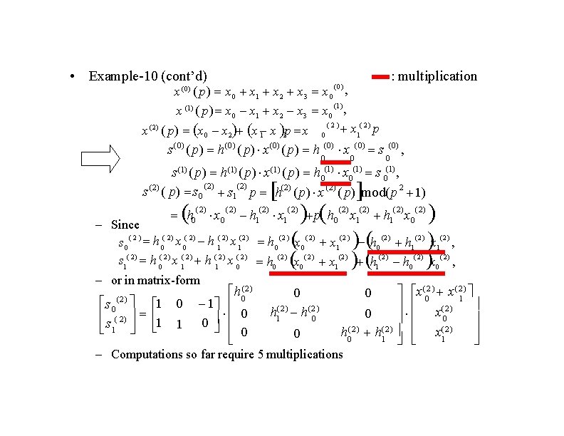
• Example-10 (cont’d) : multiplication (0 ) x ( p) x 0 x 1 x 2 x 3 x 0 , (1) x (1) ( p) x 0 x 1 x 2 x 3 x 0 , (2) ( 2) x (2) ( p) x 0 x 2 x 1 x 3 p x 0 x 1 p (0) s(0 ) ( p) h(0) ( p) x(0 ) ( p) h (0) x 0 (1) 0 (2) (0) 0 (1) 0 s (0) 0 (1) 0 , s(1) ( p) h(1) ( p) x(1) ( p) h x s , (2) s (2) ( p) s 0 s 1 p h(2 ) ( p) x ( p) mod( p 2 1) h 0 (2) x 0 (2) ( 2) h 1 x 1 (2) p h (2) (2 ) x 1 ( 2) h 1 x 0 ( 2) 0 – Since (2) ( 2) s 0 h 0 x 0 h 1 x 1 h 0 ( 2 ) x 0 ( 2) x 1( 2 ) h 0 (2) h 1 ( 2) x 1( 2 ) , s 1( 2) h 0( 2) x 1( 2) h (12) x (0 2) h 0 ( 2) x 0 ( 2 ) x 1 (2) h 1( 2 ) h 0 ( 2) x 0 ( 2) , – or in matrix-form h 0(2 ) x(02 ) x( 21) 0 0 (2) s 0 1 (2) (2) h h x 0 0 ( 2) 1 0 0 1 0 s 1 0 (2 ) (2) 1 h 0 h 1 x 1 0 – Computations so far require 5 multiplications

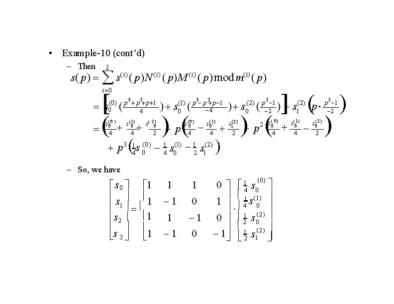
• Example-10 (cont’d) – Then 2 s( p) s (i) ( p)N (i) ( p)M (i) ( p) mod m(i) ( p) i 0 s ( (0) 0 s 0(0 ) 4 p 3 p 2 p 1 4 s(1) 0 4 s ( 20) 2 ) s ( (1) 0 p p 3 p 2 p 1 4 ) s (0 0 4 s 0(1) 4 p 3 14 s 0(0) 14 s 0(1) 12 s 1(2) p p ) s ( (2) 0 s 1(2 ) 2 p 2 1 2 s 0 1 s 1 1 s 2 1 s 3 1 1 1 1 0 ) s ( 0) 2 s 0 4 – So, we have 0 14 s 0 1 41 s (10) 0 21 s 0( 2 ) 1 (2) 1 2 s 1 ( 0) p 2 1 2 ( 2) 1 s(1) 0 4 s 0( 2 ) 2

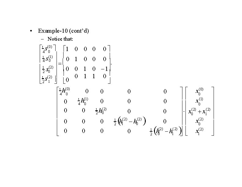
• Example-10 (cont’d) – Notice that: 14 s(0) 1 0 1 (1) 4 s 0 0 1 s 0(2) 0 12 (2) 2 s 1 0 14 h(0) 0 0 0 0 1 0 1 1 0 0 0 1 4 h(1) 0 0 1 h (2) 2 0 0 0 1 2 h 0 0 0 h 0(2) 0 (2) 1 1 2 h 0 (2) 0 h 1(2) x 0(0) (1) x 0 x 0(2) x 1(2) (2) x 0 x(2) 1

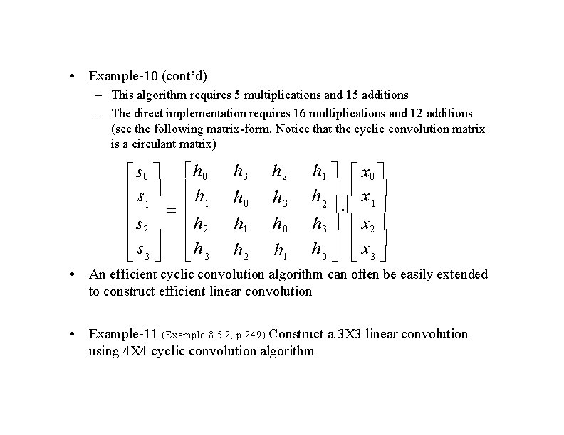
• Example-10 (cont’d) – Therefore, we have s 0 s 1 s 2 s 3 1 1 1 1 1 h 0 h 1 4 h 2 h 3 0 0 1 1 0 1 1 1 0 1 1 0 0 1 1 0 1 0 0 h 0 h 1 h 2 h 3 4 0 0 0 h 2 2 0 0 0 h 0 h 1 h 2 h 3 2 0 1 0 0 x 1 0 x 1 1 x 2 0 x 1 3 0 0 0 h 1 h 2 h 3 2 0

• Example-10 (cont’d) – This algorithm requires 5 multiplications and 15 additions – The direct implementation requires 16 multiplications and 12 additions (see the following matrix-form. Notice that the cyclic convolution matrix is a circulant matrix) s 0 h 0 s h 1 1 s 2 h 2 s 3 h 3 h 2 h 0 h 3 h 1 h 2 h 0 h 1 x 0 h 2 x 1 h 3 x 2 h 0 x 3 • An efficient cyclic convolution algorithm can often be easily extended to construct efficient linear convolution • Example-11 (Example 8. 5. 2, p. 249) Construct a 3 X 3 linear convolution using 4 X 4 cyclic convolution algorithm

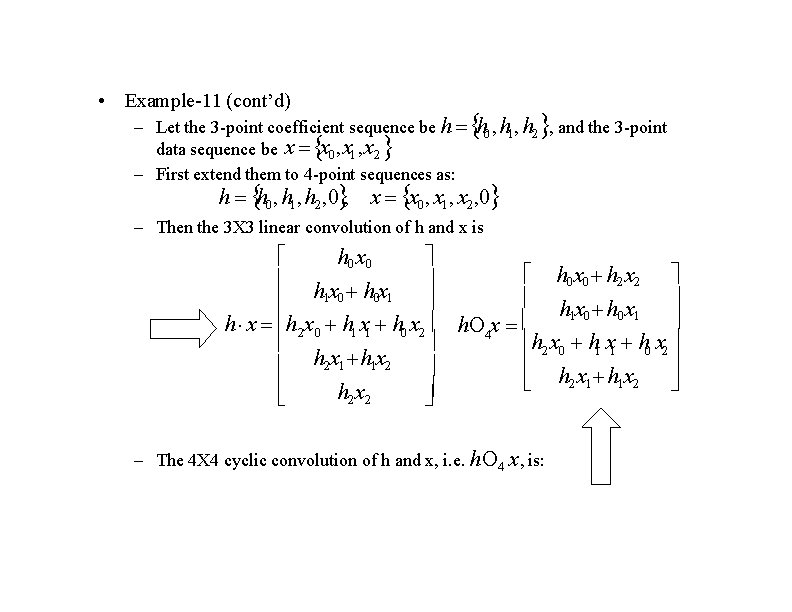
• Example-11 (cont’d) – Let the 3 -point coefficient sequence be h data sequence be x x 0 , x 1 , x 2 – First extend them to 4 -point sequences as: h 0, h 1, h 2 , and the 3 -point h h 0 , h 1, h 2 , 0 , x x 0 , x 1, x 2 , 0 – Then the 3 X 3 linear convolution of h and x is h 0 x 0 h x hx 1 0 0 1 h x h 2 x 0 h 1 x 1 h 0 x 2 h 2 x 1 h 1 x 2 h 2 x 2 h 0 x 0 h 2 x 2 h x 1 0 0 1 h 4 x h 2 x 0 h 1 x 1 h 0 x 2 h 2 x 1 h 1 x 2 – The 4 X 4 cyclic convolution of h and x, i. e. h 4 x , is:

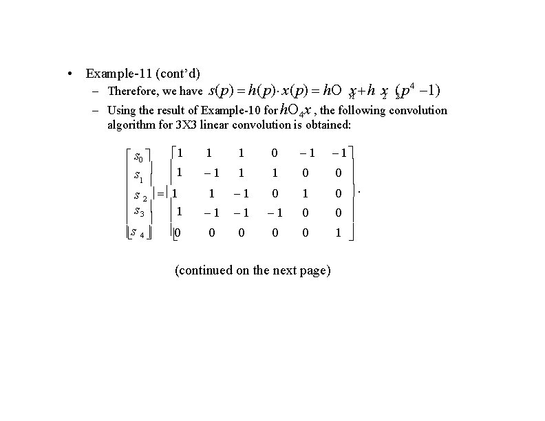
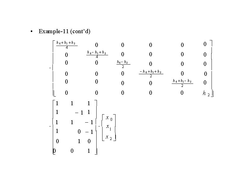
• Example-11 (cont’d) s( p) h( p) x( p) h nx h x 2 (2 p 4 1) – Using the result of Example-10 for h 4 x , the following convolution – Therefore, we have algorithm for 3 X 3 linear convolution is obtained: 1 s 0 s 1 1 s 2 1 s 3 1 0 s 4 1 1 0 1 1 1 1 0 0 0 (continued on the next page) 1 0 0 0 1

• Example-11 (cont’d) h 0 h 41 h 2 0 0 h 1 h 2 0 0 4 h 0 h 2 0 0 0 0 0 1 1 1 1 x 0 1 1 1 x 1 0 1 1 x 2 0 1 0 0 0 1 0 0 0 h 1 h 2 2 0 0 0 0 0 h 2

• Example-11 (cont’d) – So, this algorithm requires 6 multiplications and 16 additions • Comments: – In general, an efficient linear convolution can be used to obtain an efficient cyclic convolution algorithm. Conversely, an efficient cyclic convolution algorithm can be used to derive an efficient linear convolution algorithm

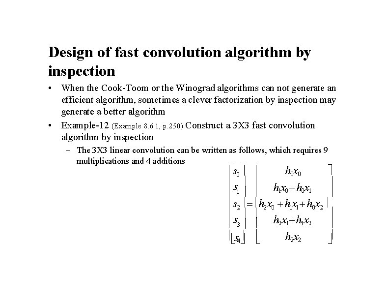
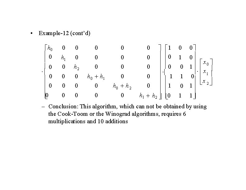
Design of fast convolution algorithm by inspection • When the Cook-Toom or the Winograd algorithms can not generate an efficient algorithm, sometimes a clever factorization by inspection may generate a better algorithm • Example-12 (Example 8. 6. 1, p. 250) Construct a 3 X 3 fast convolution algorithm by inspection – The 3 X 3 linear convolution can be written as follows, which requires 9 multiplications and 4 additions h 0 x 0 s h x 1 0 0 1 1 s 2 h 2 x 0 h 1 x 1 h 0 x 2 s h x 2 1 1 2 3 s 4 h 2 x 2

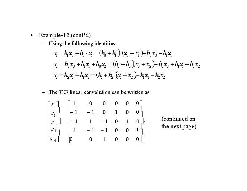
• Example-12 (cont’d) – Using the following identities: s 1 h 1 x 0 h 0 x 1 h 0 h 1 x 0 x 1 h 0 x 0 h 1 x 1 s 2 h 2 x 0 h 1 x 1 h 0 x 2 h 0 h 2 x 0 x 2 h 0 x 0 h 1 x 1 h 2 x 2 s 3 h 2 x 1 h 1 x 2 h 1 h 2 x 1 x 2 h 1 x 1 h 2 x 2 – The 3 X 3 linear convolution can be written as: 1 s 0 s 1 1 s 2 1 s 3 0 s 4 0 1 0 0 1 1 0 1 0 0 0 0 1 0 (continued on the next page)

• Example-12 (cont’d) h 0 0 0 0 0 h 1 0 0 h 2 0 0 0 0 h 0 h 1 0 0 h 0 h 2 0 0 1 0 0 0 1 0 0 0 0 1 1 0 h 1 h 2 0 1 0 0 0 x 0 1 x 1 0 x 2 1 1 – Conclusion: This algorithm, which can not be obtained by using the Cook-Toom or the Winograd algorithms, requires 6 multiplications and 10 additions