FARM MANAGEMENT Lecture 2 A Neoclassical Production Function

FARM MANAGEMENT Lecture. 2 A Neoclassical Production Function By Dr. Mahmoud Arafa Lecturer of Agricultural Economic, Cairo Un. Contacts: E-Mail: mahmoud. arafa@agr. cu. edu. eg W. S: http: //scholar. cu. edu. eg/mahmoudarafa

A neoclassical production function that uses for describing production relationships in agriculture. With this production function, as the use of input x 1 increases, the productivity of the input at first also increases.

A neoclassical production function The function turns upward, or increases, at first at an increasing rate. Then a point called the inflection point occurs. This is where the function changes from increasing at an increasing rate to increasing at a decreasing rate.

A neoclassical production function Another way of saying this is that the function is convex to the horizontal axis prior to the inflection point, but concave to the horizontal axis after the inflection point. The inflection point marks the end of increasing marginal returns and the start of diminishing marginal returns.

A neoclassical production function Finally, the function reaches a maximum and begins to turn downward. Beyond the maximum, increases in the use of the variable input x 1 result in a decrease in total output (TPP). This would occur in an instance where a farmer applied so much fertilizer that it was actually de-trimental to crop yields.

MPP for the Neoclassical Function • The MPP function changes as the use of input x 1 increases. • At first, as the productivity of input x 1 increases, so does its marginal product, and the corresponding MPP function must be increasing. • The inflection point marks the maximum marginal product. • It is here that the productivity of the incremental unit of the input x 1 is at its greatest.

MPP for the Neoclassical Function • After the inflection point, the marginal product of x 1 declines and the MPP function must also be decreasing. • The marginal product of x 1 is zero at the point of output maximization, and negative at higher levels. • Therefore, the MPP function is zero at the point of output maximization, and negative thereafter.

APP for the Neoclassical Function • Average physical product (APP) also changes as the use of x 1 increases, although APP is never negative. • As indicated earlier, APP is the ratio of output to input, in this case y/x 1 or TPP/x 1.

APP for the Neoclassical Function • Since this is the case, APP for a selected point on the production function can be illustrated by drawing a line (ray) out of the origin of the graph to the selected point. • The slope of this line is y/x 1 and corresponds to the values of y and x 1 for the production function. If the point selected on the function is for some value for x 1 called x 1*, then the APP at x 1* is y/x 1*.

• Average physical product (APP) also changes as the use of x 1 increases, although APP is never negative. As indicated earlier, APP is the ratio of output to input, in this case y/x 1 or TPP/x 1. • Call the point x 1° where y/x = dy/dx. At any point less than x 1°, the slope of the production function is greater than the slope of the line drawn from the origin to the point.

Hence APP must be less than MPP prior to x 1°. As the use of x 1 increases toward x 1°, APP increases, as does the slope of the line drawn from the origin. After x 1°, the slope of the production function is less than the slope of the line drawn from the origin to the point.

Hence MPP must be less than APP after x 1°. As the use of x 1 increases beyond x 1°, the slope of the line drawn from the origin to the point declines, and APP must decline beyond x 1°. The slope of that line never becomes negative, and APP never becomes negative.

However, a line drawn tangent to the production function represents MPP and will have a negative slope beyond the point of output maximization. APP is always non-negative, but MPP is negative beyond the point of output maximization.

The figure also illustrates the relationships that exist between the APP and the MPP function for the neoclassical production function. The MPP function first increases as the use of the input is increased, until the inflection point of the underlying production function is reached (point A).

APP for the Neoclassical Function • Average physical product (APP) also changes as the use of x 1 increases, although APP is never negative. • As indicated earlier, APP is the ratio of output to input, in this case y/x 1 or TPP/x 1.

Here the MPP function reaches its maximum. After this point, MPP declines, reaches zero when output is maximum (point C), and then turns negative. The APP function increases past the inflection point of the underlying production function until it reaches the MPP function (point B). After point B, APP declines, but never becomes negative.

The relationships that hold between APP and MPP can be proven using the composite function rule for differentiation. Notice thaty = (y/x)*x, or TPP= APP*x in the original production or TPP function dy/dx = y/x + [d(y/x)/dx]*x �� ������� �� ������ +������ �� or, equivalently MPP = APP + (slope of APP)x.

If APP is increasing and therefore has a positive slope, then MPP must be greater than APP. If APP is decreasing and therefore has a negative slope, MPP must be less than APP. If APP has a zero slope, such as would be the case where it is maximum, MPP and APP must be equal.

illustrates the TPP, The of the MPP, maximum and APP curves production function that are generated corresponds from the datato an output level of 136. 96 bushels contained in next Table. of corn per acre, using a nitrogen application rate (x) of 181. 60 pounds per acre.

The inflection point of this production function corresponding with the maximum MPP occurs at an output level of 56. 03 bushels of corn (y), with a corresponding nitrogen application rate of 60. 86 pounds per acre,

The APP maximum, where MPP intersects APP, occurs at an output level of 85. 98 bushels of corn per acre, with a corresponding nitrogen (x) application rate of 91. 30 bushels per acre.

Sign, Slope and Curvature By repeatedly differentiating a production function, it is possible to determine accurately the shape of the corresponding MPP function. For the production function y = f(x) the first derivative represents the corresponding MPP function dy/dx = f '(x) = f 1 = MPP

Insert a value for x into the function f ' (x) equation dy/dx = f '(x) = f 1 = MPP If f ' (x) (or dy/dx or MPP) is positive, then incremental units of input produce additional output. Since MPP is negative after the production function reaches its maximum, a positive sign on f ' (x) indicates that the underlying production function has a positive slope and has not yet achieved a maximum.

If f '(x) is negative, the production function is downsloping, having already achieved its maximum. The sign on the first derivative of the production function indicates if the slope of the production function is positive or negative and if MPP lies above or below the horizontal axis. If MPP is zero, then f '(x) is also zero, and the production function is likely either constant or at its maximum.

Figure illustrates seven instances where the first derivative of the TPP function is positive [(a) to (g)] f 1 = MPP; f 2 = slope of MPP; f 3 = curvature of MPP

and seven instances where the first derivative is negative [(h) to (n)]. f 1 = MPP; f 2 = slope of MPP; f 3 = curvature of MPP

• The first derivative of the TPP function could also be zero at the point where the TPP function is minimum. • The sign on the second derivative of the TPP function is used to determine if the TPP function is at a maximum or a minimum. • If the first derivative of the TPP function is zero and the second derivative is negative, the production function is at its minimum point.

If the first derivative of the TPP function is zero, and the second derivative is positive, the production function is at its minimum point. If both the first and second derivatives are zero, the function is at an inflection point, or changing from convex to the horizontal axis to concave to the horizontal axis.

However, all inflection points do not have first derivatives of zero. Finally, if the first derivative is zero and the second derivative does not exist, the production function is constant.

The second derivative of the production function is the first derivative of the MPP, or slope of the MPP function. The second derivative (d²y/dx² or f "(x) or f 2) is obtained by again differentiating the production function. d²y/dx² = f "(x) = f 2 = d. MPP/dx

If equation d²y/dx² = f "(x) = f 2 = d. MPP/dx is positive for a particular value of x, then MPP is increasing at that particular point. A negative sign indicates that MPP is decreasing at that particular point.

If f "(x) is zero, MPP is likely at a maximum at that point. In previous figure, the first derivative of the MPP function (second derivative of the TPP function) is positive in (a), (b), and (c), (l), (m), and (n); negative in (e), (f), (g), (h), (i), and (j), and zero in (d) and (k).

The second derivative of the MPP function represents the curvature of MPP and is the derivative of the original production (or TPP) function. It is obtained by again differentiating the original production function d³y/dx³ = f '" (x) = f 3 = d²MPP/dx²

The sign on f '"(x) for a particular value of x indicates the rate of change in MPP at that particular point. If MPP is in the positive quadrant and f '"(x) is positive, MPP is increasing at an increasing rate (a) as in Figure or decreasing at a decreasing rate (e).

If MPP is in the negative quadrant, a positive f '"(x) indicates that MPP is either decreasing at a decreasing rate (j) or increasing at a decreasing rate (l).

When MPP is in the positive quadrant, a negative sign on f '" (x) indicates that MPP is either increasing at a decreasing rate (c), or decreasing at an increasing rate (g). When MPP is in the negative quadrant, a negative sign on f '" (x) indicates that MPP is decreasing at an increasing rate (h) or increasing at an increasing rate (n).

If f '" (x) is zero, MPP has a constant slope with no curvature as is the case in (f), (l), and (m). If MPP is constant, f '" (x) does not exist. A similar approach might be used for APP equals y/x, and if y and x are positive, then APP must also be positive. As indicated earlier, the slope of APP is d(y/x)/dx = f '(y/x) = d APP/dx

For a particular value of x, a positive sign indicates a positive slope and a negative sign a negative slope. The curvature of APP can be represented by d²(y/x)dx² = f "(y/x) = f 2 = d²APP/dx²

For a particular value of x, a positive sign indicates that APP is increasing at an increasing rate, or decreasing at a decreasing rate. A negative sign on equation d²(y/x)dx² = f "(y/x) = f 2 = d²APP/dx² indicates that APP is increasing at a decreasing rate, or decreasing at an increasing rate. A zero indicates an APP of constant slope. The third derivative of APP would represent the rate of change in the curvature of APP.

Here are some examples of how these rules can be applied to a specific production function representing corn yield response to nitrogen fertilizer. Suppose the production function where y = corn yield in bushels per acre x = pounds of nitrogen applied per acre

For this equation, MPP is always positive for any positive level of input use, as indicated by the sign on equation MPP. If additional nitrogen is applied, some additional response in terms of increased yield will always result. If x is positive, MPP is positive and the production function has not reached a maximum.

If this equation is negative, MPP is slopes downward. Each additional pound of nitrogen that is applied will produce less and less additional corn yield. Thus the law of diminishing (MARGINAL) returns holds for this production function throughout its range.

If this equation holds, the MPP function is decreasing at a decreasing rate, coming closer and closer to the horizontal axis but never reaching or intersecting it. given that incremental pounds of nitrogen always produce a positive response in terms of additional corn.

If x is positive, APP is positive. Corn produced per pound of nitrogen fertilizer is always positive [equation If x is positive, APP is sloped downward. As the use of nitrogen increases, the average product per unit of nitrogen declines

If x is positive, APP is also decreasing at a decreasing rate. As the use of nitrogen increases, the average product per unit of nitrogen decreases but at a decreasing rate

Elasticities of Production for a Neoclassical Production Function A series of elasticities of production exist for the neoclassical production function, as a result of the relationships that exist between MPP and APP. These are illustrated in Figure.

1. The elasticity of production is greater than 1 until the point is reached where MPP = APP (point A). 2. The elasticity of production is greatest when the ratio of MPP to APP is greatest. For the neoclassical production function, this normally occurs when MPP reaches its maximum at the inflection point of the production function (point B).

3. The elasticity of production is less than 1 beyond the point where MPP = APP (point A). 4. The elasticity of production is zero when MPP is zero. Note that APP must always be positive (point C). 5. The elasticity of production is negative when MPP is negative and, of course, output is declining (beyond point C). If the production function is decreasing, MPP and the elasticity of production are negative. Again, APP must always be positive.

6. A unique characteristic of the neoclassical production function is that as the level of input use is increased, the relationship between MPP and APP is continually changing, and therefore the ratio of MPP to APP must also vary.

Further Topics on the Elasticity of Production The expression is only an approximation of the true MPP of the production function for a specific amount of the input x. The actual MPP at a specific point is better represented by inserting the value of x into the marginal product function dy/dx.

The elasticity of production for a specific level of x might be obtained by determining the value for dy/dx for that level of x and then obtaining the elasticity of production from the expression Ep = (dy/dx)*x/y

Now suppose that instead of the neoclassical production function, a simple linear relationship exists between y and x. Thus. . T PP = y = bx where b is some positive number. Then. . dy/dx = b, but note also that since y = bx, then y/x = bx/x = b. Thus MPP (dy/dx) = APP (y/x) = b. Hence, MPP/APP = b/b = 1.

The elasticity of production for any such function is 1. This means that a given percentage increase in the use of the input x will result in exactly the same percentage increase in the output y. Moreover, any production function in which the returns to the variable input are equal to some constant number will have an elasticity of production equal to 1.

Now suppose a slightly different production function Another way of writing equation is In this case And Thus, (dy/dx)/(y/x) = 0. 5

Hence the elasticity of production is 0. 5. This means that for any level of input use MPP will be precisely one half of APP. In general, the elasticity of production will be b for any production function of the form where a and b are any numbers. Notice that and that

Thus the ratio of MPP to APP-the elasticity of production- for such a function is always equal to the constant b. This is not the same as the relationship that exists between MPP and APP for the neoclassical production function in which the ratio is not constant but continually changing as the use of x increases

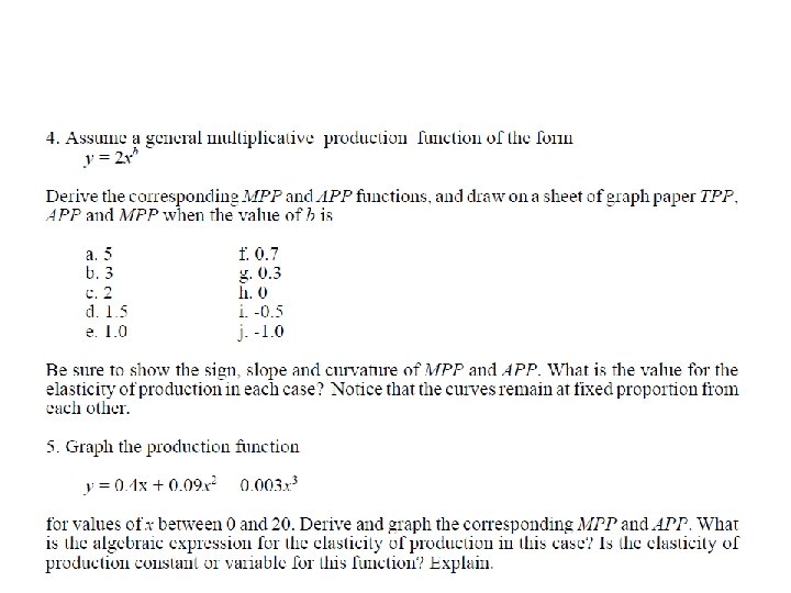
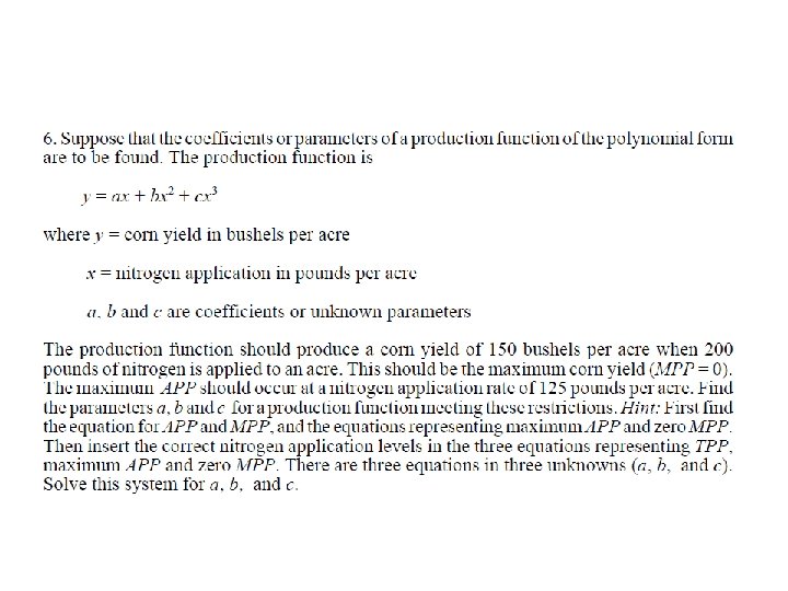
Problems and Exercises

NEXT Profit Maximization with One Input and One Output