FAO GOVERNMENT OF ITALY COOPERATIVE PROGRAMME PROJECT GCPSYR006ITA

FAO - GOVERNMENT OF ITALY COOPERATIVE PROGRAMME PROJECT GCP/SYR/006/ITA – Phase II “Assistance for Capacity Building through Enhancing Operation of the National Agricultural Policy Center” course in Partial equilibrium analysis of policy impacts Part II, September 21 – October 3, 2002 Piero Conforti - The National Institute of Agricultural Economics, Roma, Italy

Aim of this part of the course Allow the trainees to familiarise with partial equilibrium analysis of agricultural policies, within • the single market static frameworks • (hints on) multi market, dynamic PE frameworks, and on GE frameworks Special emphasis on: – price policy analysis – welfare analysis – technical change analysis Special emphasis on the applications: mostly exercises in Excel

Content 1. Equilibrium within a single market partial equilibrium computable model – isolated markets and regional integration in a closed economy with transport costs – the partial equilibrium computable model of an open economy: the effect of trade on supply demand welfare – price policy analysis: impacts on supply, demand welfare – technical change analysis with MODEXC

Content 2. Beyond the single market model – relating interdependent markets: hints on multimarket analysis in a partial equilibrium framework – hints on dynamic partial equilibrium frameworks – hints on the GE approach: basic structure, computation, calibration and estimation, applicability and limitations

Single market PE: introduction Partial equilibrium: only some parts of the economy (some markets) are taken into account. What happens in one sector in terms of demand, supply and price does not significantly affect what happens in other sectors it can be applied: to a single market (e. g. wheat) or to a set of markets (e. g. a set of agricultural products) within a socalled multi-market framework. In the second case it will take into account the interactions between e. g the wheat and the barley markets, but it will not take into account the effects of a change in the cereal market on fertilizers

Single market PE: isolated markets Three isolated regional markets with no trade; region 1: production center C production center D consumption center Y We want ot represent this in a demand-supply graph

inverted demand & supply 1. Demand derived from (1): 1 a. CPy(D) = -Dyo/Ay + Dy/Ay 2. Supply of C derived from (2) (with and without transport) 2 a. CPy = -Sco/Ac + Sc/Ac (without transport) 2 b. Cpy = (Tcy*Ac - Sco)/Ac + Sc/Ac (with transport) 3. Supply of C and D (with transport) CPy = [(Tcy*Ac+Tdy*Ad) -(Sco+Sdo)] / (Ac+Ad) + (Sc+Sd)/(Ac+Ad)

isolated market, graph We want to calculate the equilibrium point

equilibrium quantity and price production center C only Demand = Supply of C -Dyo/Ay + Dy/Ay = (Tcy*Ac-Sco)/Ac + Sc/Ac since Dy = Sc = q q = [(Tcy*Ac-Sco)/Ac) + (Dyo/Ay)] / (1/Ay - l/Ac) q= 1554 p = 361 production centers C & D Demand = Supply of C and D Dy = (Sc+Sd) = q q = {Dyo/Ay + + [(Tcy*Ac+Tdy*Ad) - (Sco+Sdo)] / (Ac+Ad)} / [(1/Ay) – l/ (Ac+Ad)] q = 1796 p =301 (from 2 a); qc = 1192 qd = 604 deducting transport costs pc = 282 pd = 276

equilibrium quantity and price Isn’t there a simpler way to calculate the equilibrium point? Yeeees!! Take the price first, instead of the quantity; consider the direct functions and solve directly for the price to get Cpy = (Dyo-Sco-Sdo+Ac*Tcy+Ad*Tdy) / (Ac+Ad-Ay)

isolated market: comments The equilibrium point is obtained when total production in the two centers equals the amount demanded by the consumers at the equilibrium price To calculate producer prices in the two areas we have to subtract the transport costs The inclusion of transport costs causes an upwards shift of the supply curve, i. e. a fixed increase in the price per each given quantity The inclusion of a second production center causes a shift of the supply curve towards the right, i. e. a change in the price-quantity relation

other regions Calculation for region 2

other regions, summary region 3, all regions

other regions, graphs Region 1 Region 3 Region 2

isolated markets, comments Prices in the isolated markets are widely different: from 146 of Region 2 to 604 of Region 3. This reflects the different production and consumption characteristics of the three regions strong production capacity in region 2 and the strong demand in 3. Isolated markets do not allow consumers of Region 3 to benefit from production capacity of Region and its low prices. Isolation can be due to natural reasons (e. g. distance, lack of communication facilities) or to political reasons (e. g. custom banners or other policies (prohibitive barriers) that eliminate trade)

market integration Suppose that region 3 and region 2 are connected by a road which allows trade region 2 region 3 A Z B X E

market integration Transport costs are given by CPz = CPx – Tzx PPa = CPx – Tzx – Taz PPb = CPx – Tzx – Tbz PPe = CPx – Tex total demand = total supply, i. e. Dx + Dz = Se + Sa + Sb where: Dx = Dxo + Ax * CPx Dz = Dzo + Az * (CPx -Tzx) Sa = Sao + Aa * (CPx- Taz- Tzx) Sb = Sbo + Ab * (CPx- Tbz- Tzx) Se = Seo + Ae * (CPx-Tex) solving for CPx

market integration we obtain

market isolation and integration, prices region 1 region 3 Y X CP = 301 CP = 604 region 2 Z CP = 146 region 1 region 3 Y X CP = 301 CP = 307 region 2 Z CP = 242 Tzx =65

market integration, comments With integration, region 3 consumes 74% more, and region 2 consumes 18% less. Price decrease by almost 50% in region 3, while it increases by almost 68% in region 2. Production increases with integration in region 2, by more than 170%, while it decreases by almost 75% in region 3. Altogethere is an increase of 22% in total consumption, and an 8. 7% decrease in production. With integration, the difference between the two prices is equal to the transport cost.

market integration, welfare effects The impact of the integration of the two markets on producers and consumers can be measured in terms of surplus. This is a money metric welfare measure With linear functions welfare changes can be approximated as (p 0 –p 1) * (d 0 +d 1) / 2 (change in consumer surplus) (p 0 –p 1) * (s 0 +s 1) / 2 (change in producer surplus) where 0 and 1 are referred to time, p is the price, s is supply and d is demand The net change in welfare is the difference between the two above (p 0 – p 1) * [(d 0 + d 1) – (s 0 + s 1)] / 2 (net gain or loss)

market integration, welfare effects Region 2 Region 3 F F D C G B A A E D B G C E In graphical terms, consumer surplus in region 2 are the areas FCB and FDE, respectively before and after market integration. The difference is CBED, which represents the losses of the consumers. The producer surplus is GCB and GAD in region 2 respectively before and after trade Since CBAD, gained by producers, is larger than CBDE, lost by consumers, trade has brought a net benefit to Region 2, equal to BEA.

market integration, welfare effects The opposite will happen in Region 3: with integration consumers will gain and producers will loose. There will be also - a transfer of income from Region 3 to Region 2, equal to the amount of purchases made by the latter in the former, and - an increase in the business of the transport sector, equal to the transport cost. Summing up, the total welfare change will be

market integration, summary of welfare effects

welfare effects, comments Altogether both region have benefited from integration, although region 3 far more than region 2. The welfare effect is unevenly distributed among social groups: consumers in region 2 and producers in region 3 suffer a loss, which is smaller than the gain of consumers in 3 and producer in 2. The first statement rests upon the hypothesis that the welfare of all social groups is directly comparable, and equally weighted.

full market integration Calculation of the equilibrium price for the three regions: supply Sc = Sco + Ac CPy – Ac Tcy Sd = Sdo + Ad CPy – Ad Tdy Sb = Sbo + Ab CPz – Ab Tbz Sa = Sao + Aa CPz – Aa Taz Se = Seo + Ae CPx – Ae Tex and given that Cpy = CPz + Tyz Cpx = CPz + Txz we have Sc = Sco + Ac CPz +Ac Tyz - Ac Tcy Sd = Sdo + Ad CPz +Ad Tyz – Ad Tdy Sb = Sbo + Ab CPz – Ab Tbz Sa = Sao + Aa CPz – Aa Taz Se = Seo + Ae CPz +Ae Txz – Ae Tex

full market integration On the demand side Dy = Dyo + Ay CPy Dz = Dzo + Az CPz Dx = Dxo + Ax CPx using the relations among regional prices: Dy = Dyo + Ay CPz + Ay Tyz Dz = Dzo + Az CPz Dx = Dxo + Ax CPz + Ax Txz thus CPz = [ - (Sco + Sdo + Seo+ Sbo + Sao) + (Dyo +Dxo + Dzo) + (Ay Tyz + Ax Txz) + + Ac (Tcy – Tyz) + Ad (Tdy – Tyz) + Ae (Tex – Txz) + Ab Tbz + Aa Taz] / / (Ac + Ad + Ae + Ab + Aa – Ay – Ax – Az)

full market integration region 3 region 1 Y X CP = 294 CP = 309 region 2 Tzy = 50 Tzx = 65 Z CP = 244

full market integration Considering also consumer prices Tcy = 19 region 1 region 3 Y X CP = 294 CP = 309 Tex = 7 C PPc = 275 E PPa = 302 Tdy = 25 Tzy = 50 Tzx = 65 region 2 D PPd = 269 Z CP = 244 Taz = 15 A PPa = 229 Tbz = 7 B PPa = 237

full market integration The gains of the consumers are greater than the losses of the producers and the costs of transport => market integration is beneficial to the country, although not for everybody.

(small) open economy: production and trade Even if fully integrated, the previous setting can be considered as being closed to foreign trade. The country has only one port of entry, in Region 3. The import price is 275 (small open). Consumers of X will prefer the imported good, which is cheaper than the local, sold at 309, this is sold at the same price of 275. Since almost 3000 tons sold in X (region 3) is coming from Z (region 2), the maximum price in Z is the price in X minus the transport cost, i. e. 210. Similarly, the price in region 1, which was also importing from region 2, will be the price of region 2 (210) plus the transportation cost of 50, i. e 260.

(small) open economy: production and trade Thus we have

closed and open economy, comparison

closed and open economy, comparison Opening to trade implies a small welfare gain for consumers, greater than the loss of the producers. The transport sector will be reduced, while foreign producers will be better off.

pan territorial prices The Government guarantees the same price to all producers and to all consumers. It has to be assumed that the Government has a Marketing Board for enforcing the price regime: this pays producers, distributes goods to the consumers, and imports. The Government sets prices equal to the average of the open market solution: producer price is 275, and consumer price is 214. The effects on production and trade

pan territorial prices

pan territorial prices

open ec and pan territorial prices, comparison Pan-territorial prices imply a net welfare loss compared to the open economy solution, despite prices were set at the same (average) levels. Moreover, the Marketing Board will suffer from a significant loss, that, in turn, will be suffered by taxpayers.

pan territorial prices, comments Administrative costs must be added to the loss of the Marketing Board, suffered by taxpayers. The implementation of this policy would not be easy: it will be difficult to impose the prices to producers and consumers. In regions 1 and 3 the it will be more profitable selling directly to the consumers, because the difference between producer and consumer price (44) is greater that the local transport cost. Similarly consumers of region 2 will find more convenient to buy the product directly from the farmers. Implementation difficulties are likely to generate additional administrative costs.

import parity prices The Government raises the producer price to the "import parity” level, e. g. to 275 for all producers in the country. This kind of provision can be adopted with several aims: e. g. • to promote an increase in the degree of self-sufficiency of the country • to support farmers income, if poor groups are mostly net food sellers. • in view of expanding the export capacity of the country. The effects on production and trade:

import parity prices

import parity prices

open ec and import parity prices, comparison The country becomes an exporter. Gains for producers are larger than losses for consumers; but the high transport costs imply a significant loss for the Marketing Board. The transport business almost doubles its revenue.

import parity prices, comments The overall welfare effect of the parity import price policy is negative, since the loss suffered by taxpayers (through the Marketing Board) are by far higher than the net welfare balance of producers and consumers. Consumption decreases by than 5. 4% in terms of expenditure, and by 11% in physical terms. This can indicate that consumers are in a condition of relative abundance, since they reduced consumption rather than substituting food with cheaper alternatives.

production and consumption subsidies The Government raises the producer price to the highest level in the country, i. e. to 268 (the level of region 3) for all producers in the country. The Government also wishes to support consumers, by fixing prices at the lowest level in the country, i. e. 210 (that of region 2). The country is a price taker, and world price is 275 This provision is adopted with the aim of supporting both agricultural producers and poor consumers, and to stimulate the growth of domestic supply. The effects on production and trade:

production and consumption subsidies

production and consumption subsidies

open ec vs prod&cons subsidies, comparison Also in this case the country becomes an exporter, there are welfare gains for both producers and consumers; but the high transport costs and the price subsidies for both producers and consumers imply a significant loss for the Marketing Board.

production and consumption subsidies, comments The overall balance of the policy is negative: the loss suffered by taxpayers (financing the Marketing Board) is greater than the net welfare gains of producers and consumers. There is a deadweight loss arising from resource misallocation. Both poduction and consumption increase significantly; in the long run this may give rise to investment in agriculture, and to further supply increases, while demand may slow down, as the population approaches satiety.

adverse weather The same simplified model can be used to analyse other phenomena, like, e. g. supply or demand shocks. An example is that of weather condition, that affect agricultural supply. Bad weather affecting production can be represented through a supply shift. The effects on production and trade:

adverse weather

adverse weather

open ec vs adverse weather, comparison In this case there is only a change in producer surplus, since consumers remain in the same position, thanks to increased imports

adverse weather, comments The small open economy hypothesis allows for prices to remain unchanged after the adverse weather: imports substitute for domestic production, thus consumer surplus does not change.

technical change In this simplified model technical change can be introduced as a supply shift, i. e. just as the opposite of the previous example of adverse weather. The effects on production and trade:

technical change

technical change

open ec vs technical change, comparison Imports in this case decreases, since more domestic production is available at the same price

technical change, comments Also in this case, the small open economy hypothesis allows for prices to remain unchanged after the technical change injection, thus consumer surplus does not change, as they substitute one to one domestically produced goods for imported ones. This means that producers get the entire benefit arising from technical change. As it will be shown, this is a very simplified representation.

beyond the static single market model Aim: providing hints on more sophisticated equilibrium modeling frameworks • MODEXC, dynamic model for the analysis of technical change • large multi market multi country frameworks employed in the analysis of agricultural policies • the functioning and the scope of general equilibrium models and CGEs

MODEXC A more sophisticated treatment compared to what was shown up to now. MODEXC: • calculates and analyzes the effects of technological change, measured as surplus of producers and consumers • allows for the treatment of different types of technical change, other than a parallel supply shift • has a slightly more sophisticated functional form • is a recursive dynamic model • assumes free market conditions and the absence of policies. It can be used for modelling both closed and (small) open economy conditions • distinguishes technical change from other supply shifters

MODEXC functional form supply demand with pm = minimum bid price p = price c, g, b = constants = own price elasticity

MODEXC dynamics Expected prices are defined according to Nerlove (1958) under a scheme of distributed lags as: where: = expected price in period "t", pt-1. . . pt-n = lagged prices from period "t-1" to period "t-n", and 1…. n = weighted factors of lagged prices.

MODEXC and tech change • The model considers technical change as a horizontal supply shift, i. e. as a percentage increase of production • if k is expressed as a percentage change of production costs (kc), it can be converted to its equivalent in terms of production expansion (kp) through supply elasticity (fp = price elasticity of supply) and with Dq = increase in production due to the new technology

MODEXC and tech change Three types of supply shift depending on the position k takes within the original function. • pivotal shift: • divergent shift: • convergent shift: The general form of shifted supply is:

Priceper unit of output MODEXC and tech change: surplus S 1 E 0 p 0 F p 1 E 1 d 0 pm p S q q 1 q Quantity of output • The area p 0 p 1 E 0 E 1 represents this gain of consumers • producers are affected by lower marginal costs (pm. FE 1) and by price reduction p 0 E 0 Fp 1; thus total producer surplus change is pm. FE 1 – p 0 E 0 Fp 1. • pm. E 0 E 1 represents the net social surplus • the final effect depends on elasticities; particularly, if demand elasticity is low producers gains are most probably small, if not negative

MODEXC and tech change The model assumes that the rate of adoption of technical change is • slow the initial stages, • then increases as the technology is more widely adopted and its performance and benefits are better known, • hen decreases in advanced stages of the adoption process, • and finally becomes stabilized This is represented assuming that the supply shift factor, k, obeys a logistic-type pattern

MODEXC and tech change The model allows to consider both supply and demand shifters, independent of thecnical change. These are demand shifter (e. g. population, income) supply shifter (tech change in other sectors) If q differs from zero, the annual k value is adjusted because q is applied on a greater base than that used to estimate the final value of k.

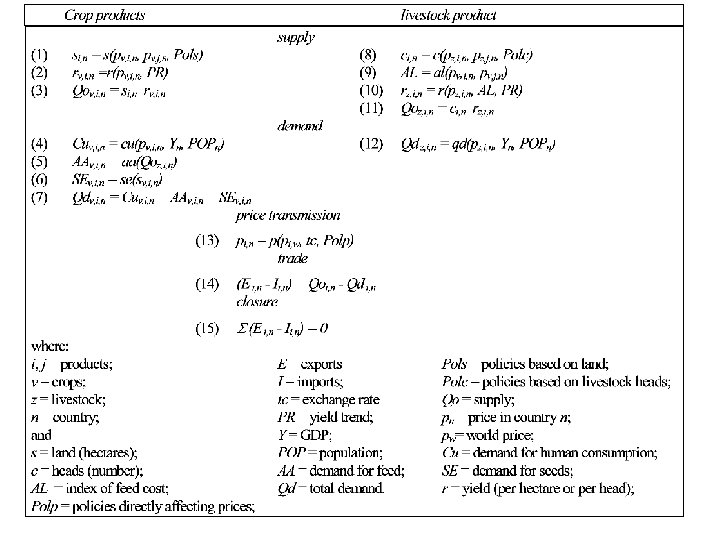
hints on large multi market PE Reference to AGLINK, FAPRI frameworks employed in agricultural policy analysis and ag market projections. A typical large PE model consists of sets of behavioral equations, equilibrium relations, and identities Equations can be grouped into a supply component, a demand or utilisation component, and a foreign trade component; This pattern is repeated for each region and product included in the models. Moreover there are price transmission equations, linking world to domestic prices, and world market equilibrium conditions that close the models.

hints on large multi market PE modeling is simplified in several respects: • production is entirely deterministic (no uncertainty factors farmers’ attitude toward risk) • input demand only for land, herds, and where primary products are employed as inputs in the production of other goods included in the model, (feed crops, oilseeds, dairy) • land use and herd depends solely on the price obtained for agricultural products. • technical change is a trend variable (rather poor representation)

hints on large multi market PE • goods produced in different countries are be perfectly homogeneous (only net trade position, no inra-industry trade) • price changes occurring in one market are always transmitted to all the other • the closure rule is defined by excess supplies, that must add up to zero in all markets • the PE assumption implies that feedbacks from agriculture to the other sectors are not described. The effects on agriculture of what happens in other sectors (and in macroeconomic variables) is usually included as exogenous shocks.

hints on large multi market PE The typical model is comparative static: it compares the two equilibrium solutions under the hypothesis that adjustment of endogenous variables is complete However, large size multi country multi commodity models often include some elements of dynamics This is modelled simply by including lagged variables in the equations, according to a recursive criteria: equilibrium solutions are based on the forecast of exogenous variables, and on the value of the endogenous variables obtained in the previous period. This implies that agents’ behaviour is optimal with reference to each single period, but not through time.

hints on GE models All productive sectors of the economy are represented. Blocks of relations dealing with production, consumption and factor use The simplest example is a setting including 2 good, 2 factors and 2 consumers

hints on GE models

hints on GE models Equilibrium conditions allow to “close” the model, and a set of identities ensure that income does not exceed expenditure, and that it equals that of the factors of production. In this simplified model only the initial factor endowments and the utility function parameter are exogenous, while all the rest is calculated by the model This can be solved by by imposing equilibrium conditions on all markets: supply (from the production functions) equals demand of the two consumers (from their utility maximisation).

GE and CGE models In order to be "computable" a general equilibrium model requires a database describing the flows of resources in the economy at the level of aggregation considered in the model; a set of parameters for the behavioral relations of the model The database for a CGE model is knonw as Social Accounting Matrix (a set of accounts describing resource flows between consumers producers, the government and foreign economies Parameters can be obtained through calibration or estimation

calibration vs estimation calibration = deterministic procedure normally used to estimate some or all parameters; the base year database is used to determine the values of the parameters that are compatible with the exogenous and the endogenous variables This does not allow a statistical control of the parameters Econometric estimation (especially through symultaneous equations) is unfeasible most of the times, due to models’ size and limited number of observations Block econometric estimation and sensitivity analysis are frequent alternatives.

advantages and drawbacks of GE vs PE approach No approach is “better” in absolute terms: all depends on the problem to be analysed Compared to the PE, the GE approach removes a simplifying hypothesis: that what happens the sector that are considered in the model do not affect demand supply in sectors that are not considered, and vice versa. Thus the GE approach can be effective to highlight the effects of a general budget constraint in the economy to consider the feedback from (e. g. ) agriculture to other sectors, and the second round effects the importance of feedback effects is related to (i) the relative size of agriculture compared to the other sectors; (ii) the degree of integration between (e. g. ) agriculture and the rest of the economy

advantages and drawbacks of GE vs PE approach. . . specifying a GE instead of a PE model appear to be worthwhile when the benefits in terms of additional information compared to the treatment of the same problem within a PE framework is greater than the increase in the “costs” associated with the time spent in data processing and the more complex specification of the mode