Faculty of Engineering Mechanical Engineering Department MATH 2140

Faculty of Engineering Mechanical Engineering Department MATH 2140 Numerical Methods Instructor: Dr. Mohamed El-Shazly Associate Prof. of Mechanical Design and Tribology melshazly@ksu. edu. sa Office: F 072

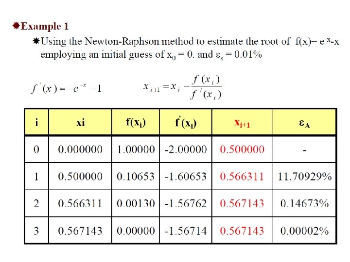
Newton-Raphson Method 2

Step 1 Evaluate 3 symbolically. http: //numericalmethods. eng. usf. edu

Step 2 Use an initial guess of the root, value of the root, , as 4 , to estimate the new http: //numericalmethods. eng. usf. edu

Step 3 Find the absolute relative approximate error 5 as http: //numericalmethods. eng. usf. edu

Step 4 Compare the absolute relative approximate error with the pre-specified relative error tolerance. Yes Is ? No Go to Step 2 using new estimate of the root. Stop the algorithm Also, check if the number of iterations has exceeded the maximum number of iterations allowed. If so, one needs to terminate the algorithm and notify the user. 6 http: //numericalmethods. eng. usf. edu

8

9

Derivation Example Convergence Final Remarks Newton’s Method Example 2: Fixed-Point Iteration & Newton’s Method Consider the function f (x ) = cos x − x = 0 Approximate a root of f using (a) a fixed-point method, and (b) Newton’s Method Numerical Analysis (Chapter 2) Newton’s Method R L Burden & J D Faires

Derivation Example Convergence Final Remarks Newton’s Method & Fixed-Point Iteration (a) Fixed-Point Iteration for f (x ) = cos x − x Numerical Analysis (Chapter 2) Newton’s Method R L Burden & J D Faires 15 / 33

Derivation Example Convergence Final Remarks Newton’s Method & Fixed-Point Iteration (a) Fixed-Point Iteration for f (x ) = cos x − x A solution to this root-finding problem is also a solution to the fixed-point problem x = cos x and the graph implies that a single fixed-point p lies in [0, π/ 2]. Numerical Analysis (Chapter 2) Newton’s Method R L Burden & J D Faires 15 / 33

Derivation Example Convergence Final Remarks Newton’s Method & Fixed-Point Iteration (a) Fixed-Point Iteration for f (x ) = cos x − x A solution to this root-finding problem is also a solution to the fixed-point problem x = cos x and the graph implies that a single fixed-point p lies in [0, π/ 2]. The following table shows the results of fixed-point iteration with p 0 = π/ 4. Numerical Analysis (Chapter 2) Newton’s Method R L Burden & J D Faires 15 / 33

Derivation Example Convergence Final Remarks Newton’s Method & Fixed-Point Iteration (a) Fixed-Point Iteration for f (x ) = cos x − x A solution to this root-finding problem is also a solution to the fixed-point problem x = cos x and the graph implies that a single fixed-point p lies in [0, π/ 2]. The following table shows the results of fixed-point iteration with p 0 = π/ 4. The best conclusion from these results is that p ≈ 0. 74. Numerical Analysis (Chapter 2) Newton’s Method R L Burden & J D Faires 15 / 33

Derivation Example Convergence Final Remarks Newton’s Method & Fixed-Point Iteration: x = cos(x ), x 0 = pn− 1 n 1 0. 7853982 2 0. 707107 3 0. 760245 4 0. 724667 5 0. 748720 6 0. 732561 7 0. 743464 Numerical Analysis (Chapter 2) pn 0. 7071068 0. 760245 0. 724667 0. 748720 0. 732561 0. 743464 0. 736128 π 4 |pn − pn− 1 | 0. 0782914 0. 053138 0. 035577 0. 024052 0. 016159 0. 010903 0. 007336 Newton’s Method en /en− 1 — 0. 678719 0. 669525 0. 676064 0. 671826 0. 674753 0. 672816 R L Burden & J D Faires

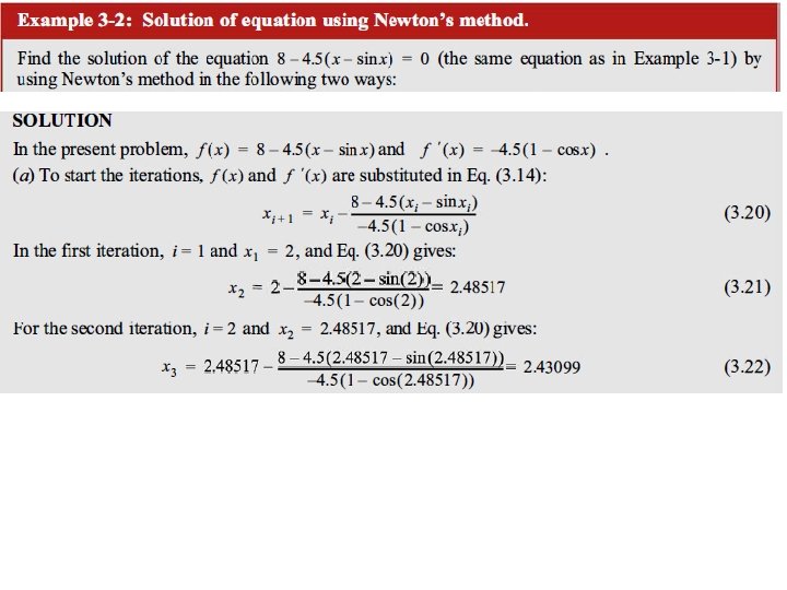
Derivation Example Convergence Final Remarks Newton’s Method (b) Newton’s Method for f (x ) = cos x − x Numerical Analysis (Chapter 2) Newton’s Method R L Burden & J D Faires 17 / 33

Derivation Example Convergence Final Remarks Newton’s Method (b) Newton’s Method for f (x ) = cos x − x To apply Newton’s method to this problem we need f t (x ) = − sin x − 1 Numerical Analysis (Chapter 2) Newton’s Method R L Burden & J D Faires 17 / 33

Derivation Example Convergence Final Remarks Newton’s Method (b) Newton’s Method for f (x ) = cos x − x To apply Newton’s method to this problem we need f t (x ) = − sin x − 1 Starting again with p 0 = π/ 4, we generate the sequence defined, for n ≥ 1, by cos pn− 1 − pn− 1 f (pn− 1) pn = pn− 1 − − sin p. f (p tn− 1 ) n− 1 Numerical Analysis (Chapter 2) Newton’s Method R L Burden & J D Faires 17 / 33

Derivation Example Convergence Final Remarks Newton’s Method (b) Newton’s Method for f (x ) = cos x − x To apply Newton’s method to this problem we need f t (x ) = − sin x − 1 Starting again with p 0 = π/ 4, we generate the sequence defined, for n ≥ 1, by cos pn− 1 − pn− 1 f (pn− 1) pn = pn− 1 − − sin p. f (p tn− 1 ) n− 1 This gives the approximations shown in the following table. Numerical Analysis (Chapter 2) Newton’s Method R L Burden & J D Faires 17 / 33

Derivation Example Convergence Final Remarks Newton’s Method for f (x ) = cos(x ) − x , x 0 = n 1 2 3 4 pn− 1 0. 78539816 0. 73953613 0. 73908518 0. 73908513 Numerical Analysis (Chapter 2) f (pn− 1 ) -0. 078291 -0. 000755 -0. 000000 f 1 (pn− 1 ) -1. 707107 -1. 673945 -1. 673612 Newton’s Method π 4 pn 0. 73953613 0. 73908518 0. 73908513 |pn − pn− 1 | 0. 04586203 0. 00045096 0. 00000004 0. 0000 R L Burden & J D Faires 18 / 33

Derivation Example Convergence Final Remarks Newton’s Method for f (x ) = cos(x ) − x , x 0 = n 1 2 3 4 pn− 1 0. 78539816 0. 73953613 0. 73908518 0. 73908513 f (pn− 1 ) -0. 078291 -0. 000755 -0. 000000 f 1 (pn− 1 ) -1. 707107 -1. 673945 -1. 673612 π 4 pn 0. 73953613 0. 73908518 0. 73908513 |pn − pn− 1 | 0. 04586203 0. 00045096 0. 00000004 0. 0000 An excellent approximation is obtained with n = 3. Numerical Analysis (Chapter 2) Newton’s Method R L Burden & J D Faires 18 / 33

Derivation Example Convergence Final Remarks Newton’s Method for f (x ) = cos(x ) − x , x 0 = n 1 2 3 4 pn− 1 0. 78539816 0. 73953613 0. 73908518 0. 73908513 f (pn− 1 ) -0. 078291 -0. 000755 -0. 000000 f 1 (pn− 1 ) -1. 707107 -1. 673945 -1. 673612 π 4 pn 0. 73953613 0. 73908518 0. 73908513 |pn − pn− 1 | 0. 04586203 0. 00045096 0. 00000004 0. 0000 An excellent approximation is obtained with n = 3. Because of the agreement of p 3 and p 4 we could reasonably expect this result to be accurate to the places listed. Numerical Analysis (Chapter 2) Newton’s Method R L Burden & J D Faires 18 / 33

Example 3 You are working for ‘DOWN THE TOILET COMPANY’ that makes floats for ABC commodes. The floating ball has a specific gravity of 0. 6 and has a radius of 5. 5 cm. You are asked to find the depth to which the ball is submerged when floating in water. Figure 3 Floating ball problem. 24

Example 3 Cont. The equation that gives the depth x in meters to which the ball is submerged under water is given by Figure 3 Floating ball problem. Use the Newton’s method of finding roots of equations to find a) the depth ‘x’ to which the ball is submerged under water. Conduct three iterations to estimate the root of the above equation. b) The absolute relative approximate error at the end of each iteration, and c) The number of significant digits at least correct at the end of each iteration. 25 http: //numericalmethods. eng. usf. edu

Example 1 Cont. Solution To aid in the understanding of how this method works to find the root of an equation, the graph of f(x) is shown to the right, where Figure 4 Graph of the function f(x) 26 http: //numericalmethods. eng. usf. edu

Example 1 Cont. Solve for Let us assume the initial guess of the root of is. This is a reasonable guess (discuss why and are not good choices) as the extreme values of the depth x would be 0 and the diameter (0. 11 m) of the ball. 27 http: //numericalmethods. eng. usf. edu

Example 1 Cont. Iteration 1 The estimate of the root is 28 http: //numericalmethods. eng. usf. edu

Example 1 Cont. Figure 5 Estimate of the root for the first iteration. http: //numericalmethods. 29 eng. usf. edu

Example 1 Cont. The absolute relative approximate error is at the end of Iteration 1 The number of significant digits at least correct is 0, as you need an absolute relative approximate error of 5% or less for at least one significant digits to be correct in your result. 30 http: //numericalmethods. eng. usf. edu

Example 1 Cont. Iteration 2 The estimate of the root is 31 http: //numericalmethods. eng. usf. edu

Example 1 Cont. Figure 6 Estimate of the root for the Iterationhttp: //numericalmethods. 2. 32 eng. usf. edu

Example 1 Cont. The absolute relative approximate error is at the end of Iteration 2 The maximum value of m for which is 2. 844. Hence, the number of significant digits at least correct in the answer is 2. 33 http: //numericalmethods. eng. usf. edu

Example 1 Cont. Iteration 3 The estimate of the root is 34 http: //numericalmethods. eng. usf. edu

Example 1 Cont. Figure 7 Estimate of the root for the Iterationhttp: //numericalmethods. 3. 35 eng. usf. edu

Example 1 Cont. The absolute relative approximate error is at the end of Iteration 3 The number of significant digits at least correct is 4, as only 4 significant digits are carried through all the calculations. 36 http: //numericalmethods. eng. usf. edu