Faculty Engineering Technology Chapter 2 Hydrology and hydraulics

| Faculty Engineering Technology Chapter 2 Hydrology and hydraulics Precipitation Najihah Abdul Rashid

Precipitation analysis Identify the type of precipitation and the methods of measurement

Precipitation • water (solid, liquid) falling from atmosphere to ground • Include rain, drizzle, snow, hail, sleet, ice crystals • Magnitude of rain is varies depend on time and location • Conditions: – – Humid Nuclei Droplets to raindrops Size of raindrops • Adiabatic expansion due to pressure change

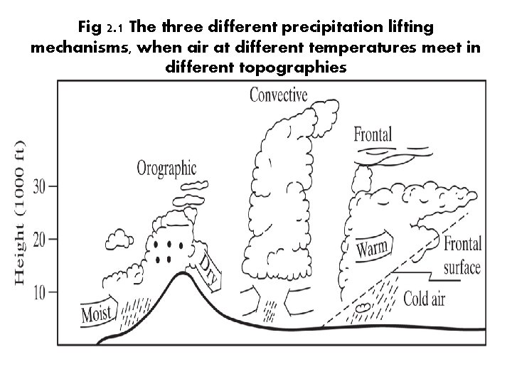
Formation of precipitation Different topographies • Convective: due to intense heating of air on the ground causes to expansion and vertical rise of air • Cyclonic: movement of large air-mass system (warm or cold fronts) • Orographic: due to mechanical lifting of moist air masses over the windward side of mountain ranges

Fig 2. 1 The three different precipitation lifting mechanisms, when air at different temperatures meet in different topographies

Precipitation measurement • Container to collect P in a storm event • Radar, digital recorders • Accuracy depends on physical setting, disturbances… etc • Weather data available from government agencies

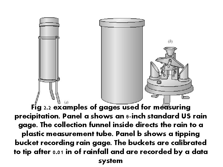
Fig 2. 2 examples of gages used for measuring precipitation. Panel a shows an 8 -inch standard US rain gage. The collection funnel inside directs the rain to a plastic measurement tube. Panel b shows a tipping bucket recording rain gage. The buckets are calibrated to tip after 0. 01 in of rainfall and are recorded by a data system

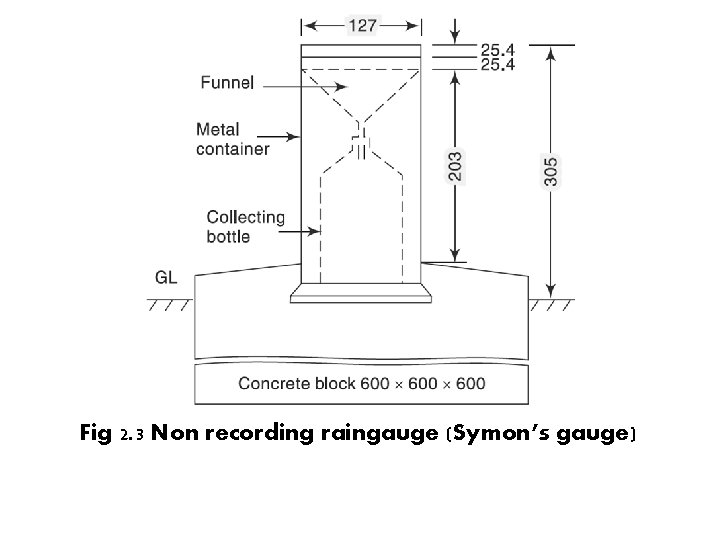
Precipitation measurement (cont) • Standard settings are adopted to accurately represent the rainfall in the area surrounding the raingauge. • Standard settings – The ground must be level and in the open and the instrument must be present a horizontal catch surface – Must be set near the ground to reduce wind effects but must be sufficiently high to prevent splashing, flooding etc – Surrounded by an open fenced area of at least 5. 5 m x 5. 5 m. No object should be nearer to the instrument than 30 m or twice the height of the obstruction

Fig 2. 3 Non recording raingauge (Symon’s gauge)

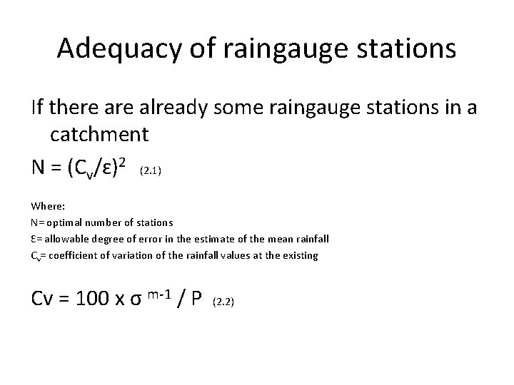
Adequacy of raingauge stations If there already some raingauge stations in a catchment N = (Cv/ɛ)2 (2. 1) Where: N= optimal number of stations Ɛ= allowable degree of error in the estimate of the mean rainfall Cv= coefficient of variation of the rainfall values at the existing Cv = 100 x σ m-1 / P (2. 2)

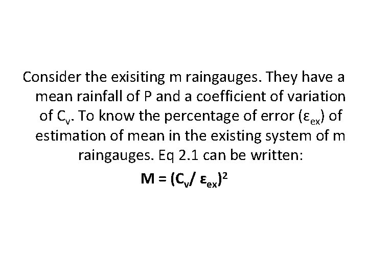
Consider the exisiting m raingauges. They have a mean rainfall of P and a coefficient of variation of Cv. To know the percentage of error (ɛex) of estimation of mean in the existing system of m raingauges. Eq 2. 1 can be written: M = (Cv/ ɛex)2

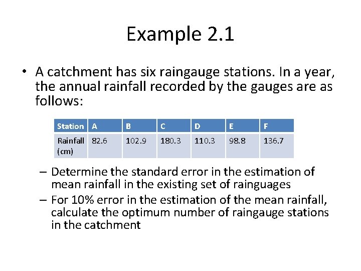
Example 2. 1 • A catchment has six raingauge stations. In a year, the annual rainfall recorded by the gauges are as follows: Station A B C D E F Rainfall 82. 6 (cm) 102. 9 180. 3 110. 3 98. 8 136. 7 – Determine the standard error in the estimation of mean rainfall in the existing set of rainguages – For 10% error in the estimation of the mean rainfall, calculate the optimum number of raingauge stations in the catchment

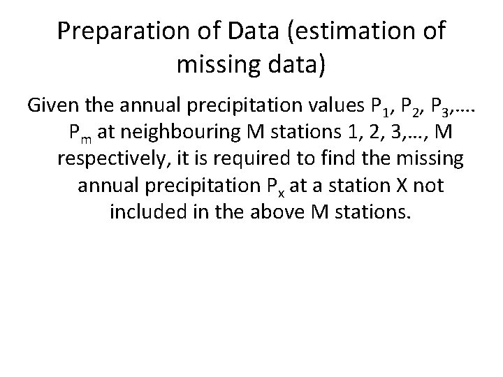
Preparation of Data (estimation of missing data) Given the annual precipitation values P 1, P 2, P 3, …. Pm at neighbouring M stations 1, 2, 3, …, M respectively, it is required to find the missing annual precipitation Px at a station X not included in the above M stations.

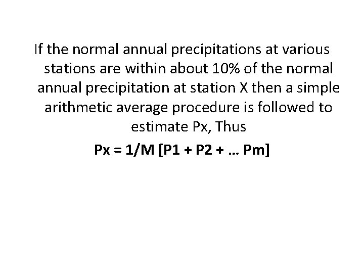
If the normal annual precipitations at various stations are within about 10% of the normal annual precipitation at station X then a simple arithmetic average procedure is followed to estimate Px, Thus Px = 1/M [P 1 + P 2 + … Pm]

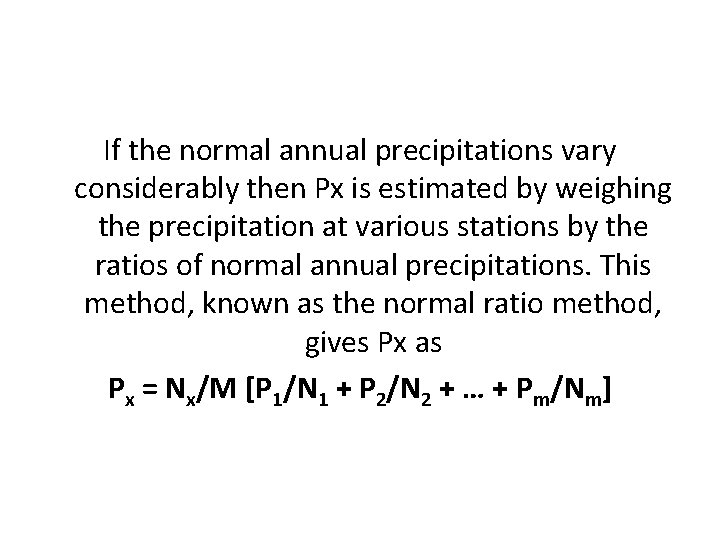
If the normal annual precipitations vary considerably then Px is estimated by weighing the precipitation at various stations by the ratios of normal annual precipitations. This method, known as the normal ratio method, gives Px as Px = Nx/M [P 1/N 1 + P 2/N 2 + … + Pm/Nm]

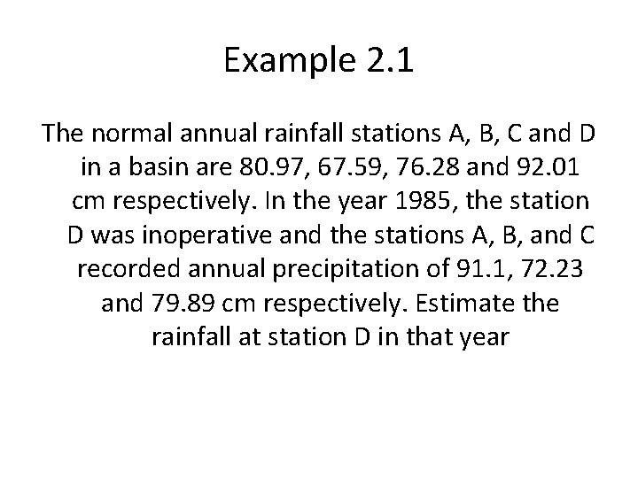
Example 2. 1 The normal annual rainfall stations A, B, C and D in a basin are 80. 97, 67. 59, 76. 28 and 92. 01 cm respectively. In the year 1985, the station D was inoperative and the stations A, B, and C recorded annual precipitation of 91. 1, 72. 23 and 79. 89 cm respectively. Estimate the rainfall at station D in that year

Test for consistency of record If the conditions relevant to the recording of a raingauge station have undergone a significant change during the period of record, inconsistency would arise in the rainfall data of that station

• Some of the common causes for inconsistency of record are – Shifting a raingauge station to a new location – The neighbourhood of the station undergoing a marked change – Change in the ecosystem – Occurrence of observational error

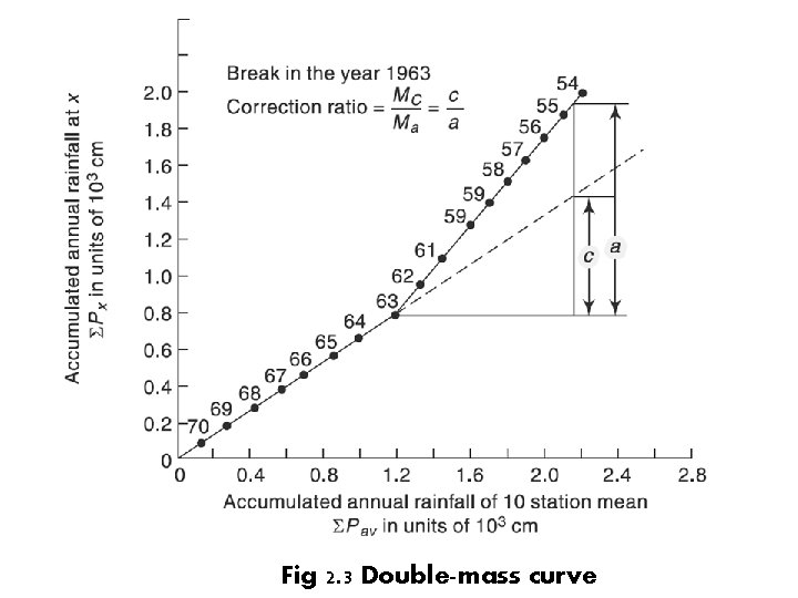
Fig 2. 3 Double-mass curve

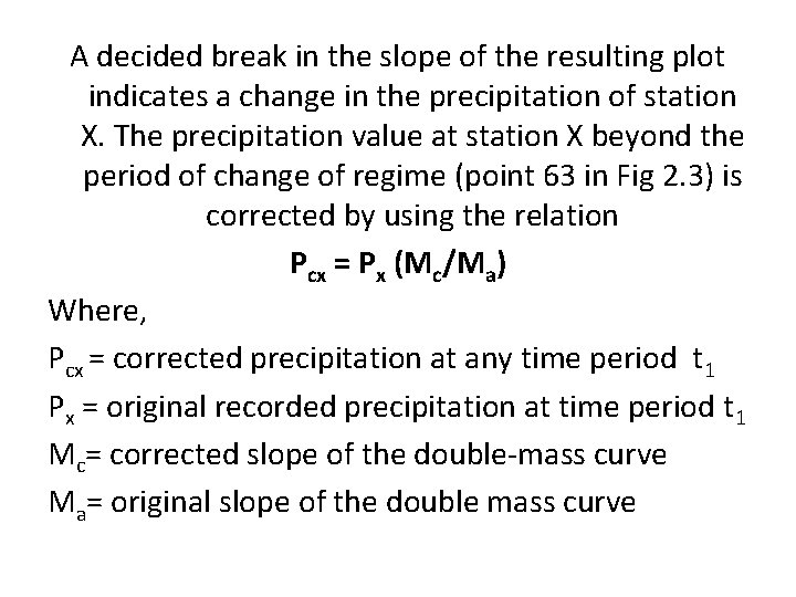
A decided break in the slope of the resulting plot indicates a change in the precipitation of station X. The precipitation value at station X beyond the period of change of regime (point 63 in Fig 2. 3) is corrected by using the relation Pcx = Px (Mc/Ma) Where, Pcx = corrected precipitation at any time period t 1 Px = original recorded precipitation at time period t 1 Mc= corrected slope of the double-mass curve Ma= original slope of the double mass curve

Example 2. 2 Annual rainfall data for station M as well as the average annual rainfall values for a group of ten neighbouring stations located in a meteorologically homogeneous region are give (see attachment)

Solution 2. 2 The data is sorted in descending order of the year, starting from the latest year 1979. Cumulative values of station M rainfall (ƩPm) and the ten station average rainfall values (ƩPav) are calculated. The data is then plotted with ƩPm on the y-axis and ƩPav on the x-axis

Presentation of rainfall data • • Mass curve of rainfall Hyetograph Point rainfall Moving average

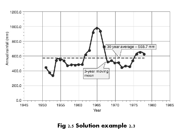
Moving average Technique for smoothening out the high frequency fluctuations of a time series and to enable the trend, if any to be noticed. The basic principle is that window of time range m years is selected. Starting from the first set of m years of data, the average of the data for m years is calculated and placed in the middle year of the range m. the window is next moved sequentially

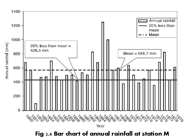
Example 2. 3 Annual rainfall values recorded at station M for the period 1950 to 1979 is given in attachment. Represent this data as a bar diagram with time in chronological order

Fig 2. 4 Bar chart of annual rainfall at station M

Fig 2. 5 Solution example 2. 3

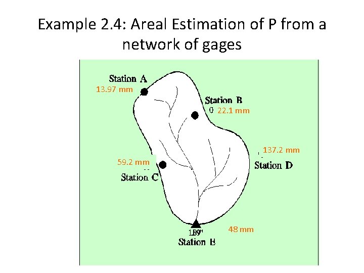
Mean precipitation over an area Arithmetic average: for evenly distribute stations (uniform density) Thiessen method area-weighted averaging Isohyetal lines contouring

Example 2. 4: Areal Estimation of P from a network of gages 13. 97 mm 22. 1 mm 137. 2 mm 59. 2 mm 48 mm

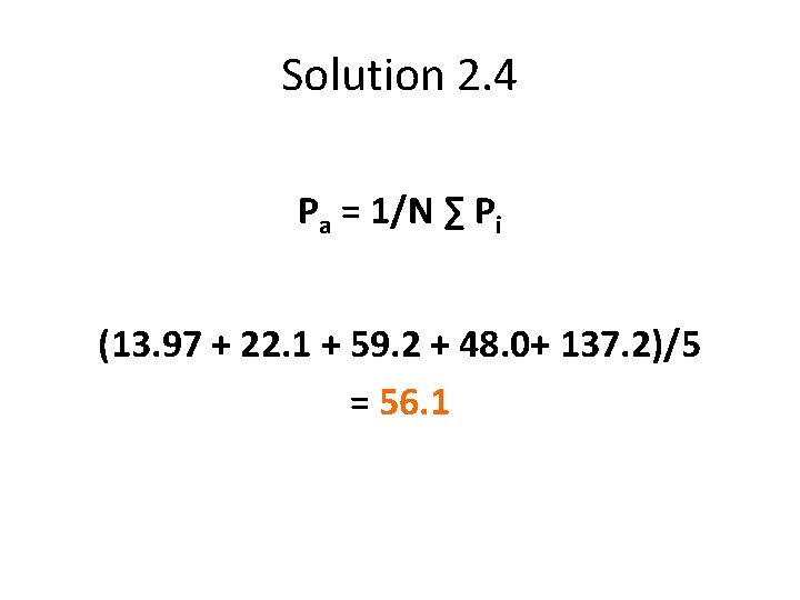
Solution 2. 4 Pa = 1/N ∑ Pi (13. 97 + 22. 1 + 59. 2 + 48. 0+ 137. 2)/5 = 56. 1

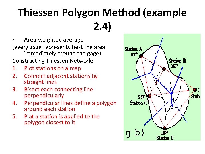
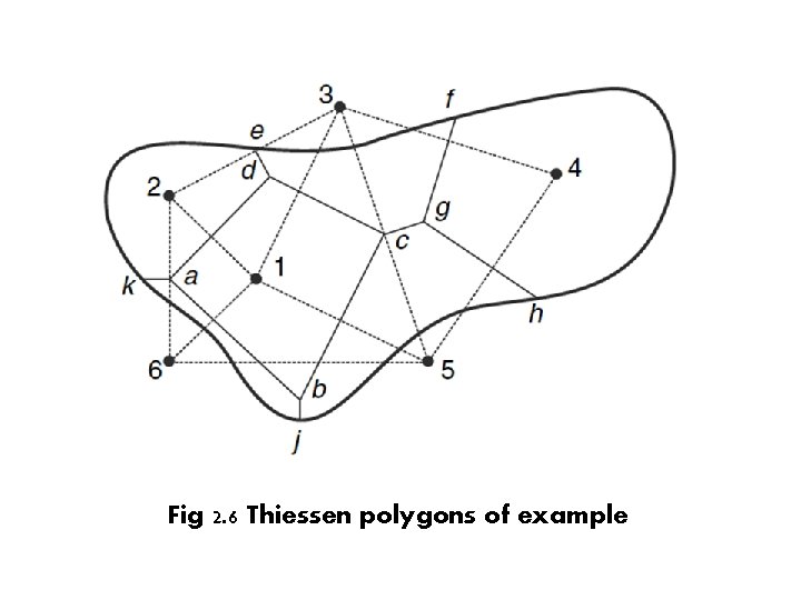
Thiessen Polygon Method (example 2. 4) • Area-weighted average (every gage represents best the area immediately around the gage) Constructing Thiessen Network: 1. Plot stations on a map 2. Connect adjacent stations by straight lines 3. Bisect each connecting line perpendicularly 4. Perpendicular lines define a polygon around each station 5. P at a station is applied to the polygon closest to it

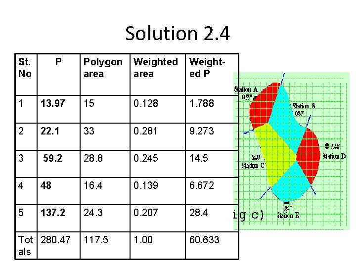
Solution 2. 4 St. No P Polygon area Weighted P 1 13. 97 15 0. 128 1. 788 2 22. 1 33 0. 281 9. 273 3 59. 2 28. 8 0. 245 14. 5 4 48 16. 4 0. 139 6. 672 5 137. 2 24. 3 0. 207 28. 4 117. 5 1. 00 60. 633 Tot 280. 47 als

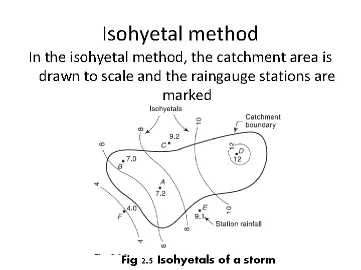
Isohyetal method In the isohyetal method, the catchment area is drawn to scale and the raingauge stations are marked Fig 2. 5 Isohyetals of a storm

Fig 2. 6 Thiessen polygons of example

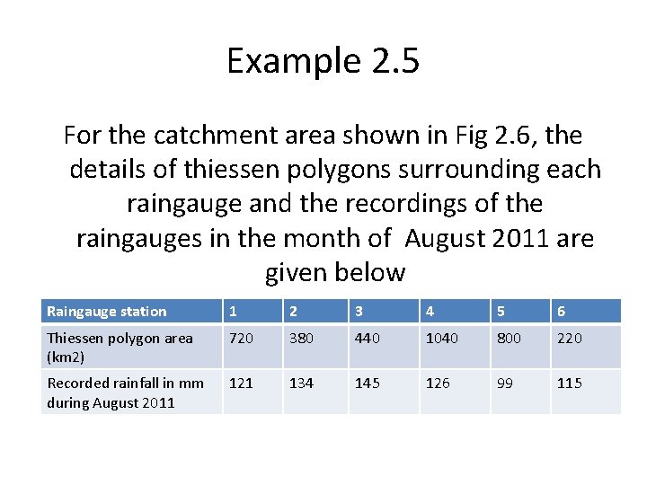
Example 2. 5 For the catchment area shown in Fig 2. 6, the details of thiessen polygons surrounding each raingauge and the recordings of the raingauges in the month of August 2011 are given below Raingauge station 1 2 3 4 5 6 Thiessen polygon area (km 2) 720 380 440 1040 800 220 Recorded rainfall in mm during August 2011 121 134 145 126 99 115

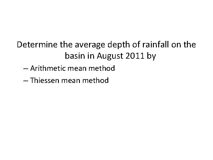
Determine the average depth of rainfall on the basin in August 2011 by – Arithmetic mean method – Thiessen mean method

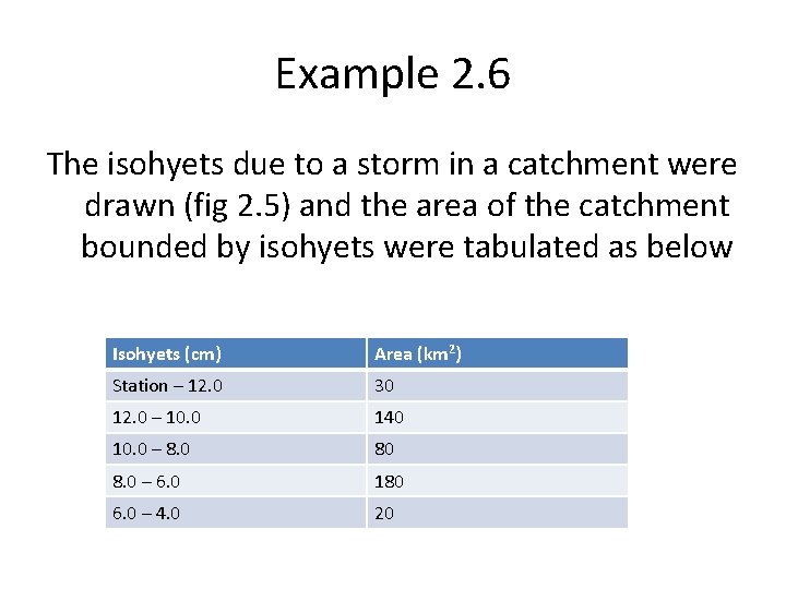
Example 2. 6 The isohyets due to a storm in a catchment were drawn (fig 2. 5) and the area of the catchment bounded by isohyets were tabulated as below Isohyets (cm) Area (km 2) Station – 12. 0 30 12. 0 – 10. 0 140 10. 0 – 8. 0 80 8. 0 – 6. 0 180 6. 0 – 4. 0 20

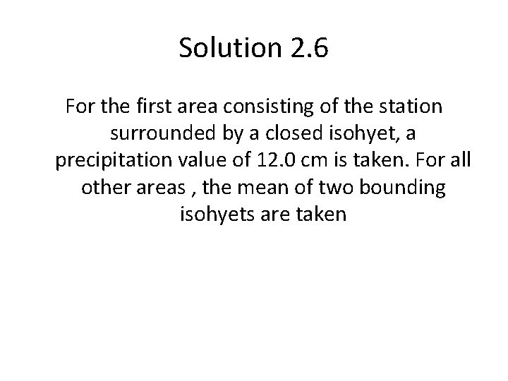
Solution 2. 6 For the first area consisting of the station surrounded by a closed isohyet, a precipitation value of 12. 0 cm is taken. For all other areas , the mean of two bounding isohyets are taken