Factorial Experiments Analysis of Variance Experimental Design Dependent

Factorial Experiments Analysis of Variance Experimental Design

• Dependent variable Y • k Categorical independent variables A, B, C, … (the Factors) • Let – a = the number of categories of A – b = the number of categories of B – c = the number of categories of C – etc.

The Completely Randomized Design • We form the set of all treatment combinations – the set of all combinations of the k factors • Total number of treatment combinations – t = abc…. • In the completely randomized design n experimental units (test animals , test plots, etc. are randomly assigned to each treatment combination. – Total number of experimental units N = nt=nabc. .

The treatment combinations can thought to be arranged in a k-dimensional rectangular block 1 1 2 A a 2 B b

C B A

Another way of representing the treatment combinations in a factorial experiment C B . . . A . . . D

Example In this example we are examining the effect of The level of protein A (High or Low) and The source of protein B (Beef, Cereal, or Pork) on weight gains Y (grams) in rats. We have n = 10 test animals randomly assigned to k = 6 diets

The k = 6 diets are the 6 = 3× 2 Level-Source combinations 1. High - Beef 2. High - Cereal 3. High - Pork 4. Low - Beef 5. Low - Cereal 6. Low - Pork

Table Gains in weight (grams) for rats under six diets differing in level of protein (High or Low) and s ource of protein (Beef, Cereal, or Pork) Level of Protein High Protein Low protein Source of Protein Beef Cereal Pork Diet 1 2 3 4 5 6 73 98 94 90 107 49 102 74 79 76 95 82 118 56 96 90 97 73 104 111 98 64 80 86 81 95 102 86 98 81 107 88 102 51 74 97 100 82 108 72 74 106 87 77 91 90 67 70 117 86 120 95 89 61 111 92 105 78 58 82 Mean 100. 0 85. 9 99. 5 79. 2 83. 9 78. 7 Std. Dev. 15. 14 15. 02 10. 92 13. 89 15. 71 16. 55

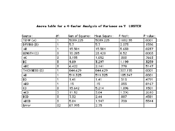
Example – Four factor experiment Four factors are studied for their effect on Y (luster of paint film). The four factors are: 1) Film Thickness - (1 or 2 mils) 2) Drying conditions (Regular or Special) 3) Length of wash (10, 30, 40 or 60 Minutes), and 4) Temperature of wash (92 ˚C or 100 ˚C) Two observations of film luster (Y) are taken for each treatment combination

The data is tabulated below: Regular Dry Minutes 92 C 1 -mil Thickness 20 3. 4 30 4. 1 40 4. 9 4. 2 60 5. 0 4. 9 2 -mil Thickness 20 5. 5 3. 7 30 5. 7 6. 1 40 5. 5 5. 6 60 7. 2 6. 0 100 C 92 C Special Dry 100 C 19. 6 17. 5 17. 6 20. 9 14. 5 17. 0 15. 2 17. 1 2. 1 4. 0 5. 1 8. 3 3. 8 4. 6 3. 3 4. 3 17. 2 13. 5 16. 0 17. 5 13. 4 14. 3 17. 8 13. 9 26. 6 31. 6 30. 5 29. 5 30. 2 4. 5 5. 9 5. 5 5. 8 25. 6 29. 2 32. 6 22. 5 29. 8 27. 4 31. 4 29. 6 8. 0 9. 9 33. 5 29. 5

Notation Let the single observations be denoted by a single letter and a number of subscripts yijk…. . l The number of subscripts is equal to: (the number of factors) + 1 1 st subscript = level of first factor 2 nd subscript = level of 2 nd factor … Last subsrcript denotes different observations on the same treatment combination

Notation for Means When averaging over one or several subscripts we put a “bar” above the letter and replace the subscripts by • Example: y 241 • •

Profile of a Factor Plot of observations means vs. levels of the factor. The levels of the other factors may be held constant or we may average over the other levels

Definition: A factor is said to not affect the response if the profile of the factor is horizontal for all combinations of levels of the other factors: No change in the response when you change the levels of the factor (true for all combinations of levels of the other factors) Otherwise the factor is said to affect the response:

Definition: • Two (or more) factors are said to interact if changes in the response when you change the level of one factor depend on the level(s) of the other factor(s). • Profiles of the factor for different levels of the other factor(s) are not parallel • Otherwise the factors are said to be additive . • Profiles of the factor for different levels of the other factor(s) are parallel.

• If two (or more) factors interact each factor effects the response. • If two (or more) factors are additive it still remains to be determined if the factors affect the response • In factorial experiments we are interested in determining – which factors effect the response and – which groups of factors interact.

Factor A has no effect B A

Additive Factors B A

Interacting Factors B A

The testing in factorial experiments 1. Test first the higher order interactions. 2. If an interaction is present there is no need to test lower order interactions or main effects involving those factors. All factors in the interaction affect the response and they interact 3. The testing continues with for lower order interactions and main effects for factors which have not yet been determined to affect the response.

Example: Diet Example Summary Table of Cell means Source of Protein Level of Protein Beef High 100. 00 Low 79. 20 Overall 89. 60 Cereal 85. 90 83. 90 84. 90 Pork Overall 99. 50 95. 13 78. 70 80. 60 89. 10 87. 87

Profiles of Weight Gain for Source and Level of Protein

Profiles of Weight Gain for Source and Level of Protein

Models for factorial Experiments Single Factor: A – a levels Random error – Normal, mean 0, std-dev. s yij = m + ai + eij Overall mean i = 1, 2, . . . , a; j = 1, 2, . . . , n Effect on y of factor A when A = i

1 observations Levels of A 2 3 a y 11 y 12 y 13 y 21 y 22 y 23 y 31 y 32 y 33 ya 1 ya 2 ya 3 y 1 n y 2 n y 3 n yan m 1 m 2 Normal dist’n Mean of observations Definitions m + a 1 m + a 2 m 3 m + a 3 ma m + aa

Two Factor: A (a levels), B (b levels yijk = m + ai + bj+ (ab)ij + eijk i = 1, 2, . . . , a ; j = 1, 2, . . . , b ; k = 1, 2, . . . , n Overall mean Main effect of A Main effect of B Interaction effect of A and B

Table of Means

Table of Effects – Overall mean, Main effects, Interaction Effects

Three Factor: A (a levels), B (b levels), C (c levels) yijkl = m + ai + bj+ (ab)ij + gk + (ag)ik + (bg)jk+ (abg)ijk + eijkl = m + ai + bj+ gk + (ab)ij + (ag)ik + (bg)jk Main effects + (abg)ijk + eijkl Two factor Interactions Three factor Interaction Random error i = 1, 2, . . . , a ; j = 1, 2, . . . , b ; k = 1, 2, . . . , c; l = 1, 2, . . . , n

mijk = the mean of y when A = i, B = j, C = k = m + ai + bj+ gk + (ab)ij + (ag)ik + (bg)jk + (abg)ijk Two factor Overall mean Main effects Three factor Interactions i = 1, 2, . . . , a ; j = 1, 2, . . . , b ; k = 1, 2, . . . , c; l = 1, 2, . . . , n

No interaction Levels of C Levels of B Levels of A

A, B interact, No interaction with C Levels of B Levels of A

A, B, C interact Levels of C Levels of B Levels of A

Four Factor: yijklm = m + ai + bj+ (ab)ij + gk + (ag)ik + (bg)jk+ (abg)ijk + dl+ (ad)il + (bd)jl+ (abd)ijl + (gd)kl + (agd)ikl + (bgd)jkl+ (abgd)ijkl + eijklm Overall mean =m Two factor Main effects + a i + b j + gk + dl Interactions + (ab)ij + (ag)ik + (bg)jk + (ad)il + (bd)jl+ (gd)kl +(abg)ijk+ (abd)ijl + (agd)ikl + (bgd)jkl Three factor Interactions + (abgd)ijkl + eijklm Four factor Interaction Random error i = 1, 2, . . . , a ; j = 1, 2, . . . , b ; k = 1, 2, . . . , c; l = 1, 2, . . . , d; m = 1, 2, . . . , n where 0 = S ai = S bj= S (ab)ij = S gk = S (ag)ik = S(bg)jk= S (abg)ijk = S dl= S (ad)il = S (bd)jl = S (abd)ijl = S (gd)kl = S (agd)ikl = S (bgd)jkl = S (abgd)ijkl and S denotes the summation over any of the subscripts.

Estimation of Main Effects and Interactions • Estimator of Main effect of a Factor = Mean at level i of the factor - Overall Mean • Estimator of k-factor interaction effect at a combination of levels of the k factors = Mean at the combination of levels of the k factors - sum of all means at k-1 combinations of levels of the k factors +sum of all means at k-2 combinations of levels of the k factors - etc.

Example: • The main effect of factor B at level j in a four factor (A, B, C and D) experiment is estimated by: • The two-factor interaction effect between factors B and C when B is at level j and C is at level k is estimated by:

• The three-factor interaction effect between factors B, C and D when B is at level j, C is at level k and D is at level l is estimated by: • Finally the four-factor interaction effect between factors A, B, C and when A is at level i, B is at level j, C is at level k and D is at level l is estimated by:

Anova Table entries • Sum of squares interaction (or main) effects being tested = (product of sample size and levels of factors not included in the interaction) × (Sum of squares of effects being tested) • Degrees of freedom = df = product of (number of levels - 1) of factors included in the interaction.

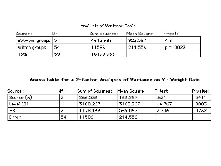
Analysis of Variance (ANOVA) Table Entries (Two factors – A and B)

The ANOVA Table

Analysis of Variance (ANOVA) Table Entries (Three factors – A, B and C)

The ANOVA Table

• The Completely Randomized Design is called balanced • If the number of observations per treatment combination is unequal the design is called unbalanced. (resulting mathematically more complex analysis and computations) • If for some of the treatment combinations there are no observations the design is called incomplete. (some of the parameters - main effects and interactions - cannot be estimated. )

Example: Diet example Mean = 87. 867

Main Effects for Factor A (Source of Protein) Beef 1. 733 Cereal -2. 967 Pork 1. 233

Main Effects for Factor B (Level of Protein) High 7. 267 Low -7. 267

AB Interaction Effects Source of Protein Beef Cereal Pork Level High 3. 133 -6. 267 3. 133 of Protein Low -3. 133 6. 267 -3. 133

Example 2 Paint Luster Experiment

Table: Means and Cell Frequencies

Means and Frequencies for the AB Interaction (Temp - Drying)

Profiles showing Temp-Dry Interaction

Means and Frequencies for the AD Interaction (Temp- Thickness)

Profiles showing Temp-Thickness Interaction

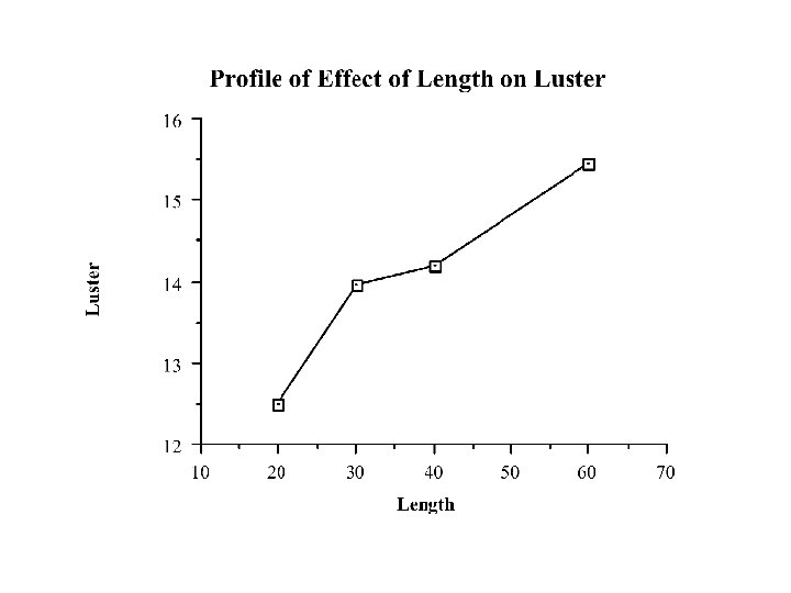
The Main Effect of C (Length)

Factorial Experiments Analysis of Variance Experimental Design

• Dependent variable Y • k Categorical independent variables A, B, C, … (the Factors) • Let – a = the number of categories of A – b = the number of categories of B – c = the number of categories of C – etc.

Objectives • Determine which factors have some effect on the response • Which groups of factors interact

The Completely Randomized Design • We form the set of all treatment combinations – the set of all combinations of the k factors • Total number of treatment combinations – t = abc…. • In the completely randomized design n experimental units (test animals , test plots, etc. are randomly assigned to each treatment combination. – Total number of experimental units N = nt=nabc. .

Factor A has no effect B A

Additive Factors B A

Interacting Factors B A

The testing in factorial experiments 1. Test first the higher order interactions. 2. If an interaction is present there is no need to test lower order interactions or main effects involving those factors. All factors in the interaction affect the response and they interact 3. The testing continues with for lower order interactions and main effects for factors which have not yet been determined to affect the response.

Anova table for the 3 factor Experiment Source SS df MS F A SSA a-1 MSA/MSError B SSB b-1 MSB/MSError C SSC c-1 MSC/MSError AB SSAB (a - 1)(b - 1) MSAB/MSError AC SSAC (a - 1)(c - 1) MSAC/MSError BC SSBC (b - 1)(c - 1) MSBC/MSError ABC SSABC (a - 1)(b - 1)(c - 1) MSABC/MSError SSError abc(n - 1) MSError p -value

Sum of squares entries Similar expressions for SSB , and SSC. Similar expressions for SSBC , and SSAC.

Sum of squares entries Finally

The statistical model for the 3 factor Experiment

Anova table for the 3 factor Experiment Source SS df MS F A SSA a-1 MSA/MSError B SSB b-1 MSB/MSError C SSC c-1 MSC/MSError AB SSAB (a - 1)(b - 1) MSAB/MSError AC SSAC (a - 1)(c - 1) MSAC/MSError BC SSBC (b - 1)(c - 1) MSBC/MSError ABC SSABC (a - 1)(b - 1)(c - 1) MSABC/MSError SSError abc(n - 1) MSError p -value

The testing in factorial experiments 1. Test first the higher order interactions. 2. If an interaction is present there is no need to test lower order interactions or main effects involving those factors. All factors in the interaction affect the response and they interact 3. The testing continues with lower order interactions and main effects for factors which have not yet been determined to affect the response.

Examples Using SPSS

Example In this example we are examining the effect of • the level of protein A (High or Low) and • the source of protein B (Beef, Cereal, or Pork) on weight gains (grams) in rats. We have n = 10 test animals randomly assigned to k = 6 diets

The k = 6 diets are the 6 = 3× 2 Level-Source combinations 1. High - Beef 2. High - Cereal 3. High - Pork 4. Low - Beef 5. Low - Cereal 6. Low - Pork

Table Gains in weight (grams) for rats under six diets differing in level of protein (High or Low) and s ource of protein (Beef, Cereal, or Pork) Level of Protein High Protein Low protein Source of Protein Beef Cereal Pork Diet 1 2 3 4 5 6 73 98 94 90 107 49 102 74 79 76 95 82 118 56 96 90 97 73 104 111 98 64 80 86 81 95 102 86 98 81 107 88 102 51 74 97 100 82 108 72 74 106 87 77 91 90 67 70 117 86 120 95 89 61 111 92 105 78 58 82 Mean 100. 0 85. 9 99. 5 79. 2 83. 9 78. 7 Std. Dev. 15. 14 15. 02 10. 92 13. 89 15. 71 16. 55

The data as it appears in SPSS

To perform ANOVA select Analyze->General Linear Model-> Univariate

The following dialog box appears

Select the dependent variable and the fixed factors Press OK to perform the Analysis

The Output

Example – Four factor experiment Four factors are studied for their effect on Y (luster of paint film). The four factors are: 1) Film Thickness - (1 or 2 mils) 2) Drying conditions (Regular or Special) 3) Length of wash (10, 30, 40 or 60 Minutes), and 4) Temperature of wash (92 ˚C or 100 ˚C) Two observations of film luster (Y) are taken for each treatment combination

The data is tabulated below: Regular Dry Minutes 92 C 1 -mil Thickness 20 3. 4 30 4. 1 40 4. 9 4. 2 60 5. 0 4. 9 2 -mil Thickness 20 5. 5 3. 7 30 5. 7 6. 1 40 5. 5 5. 6 60 7. 2 6. 0 100 C 92 C Special Dry 100 C 19. 6 17. 5 17. 6 20. 9 14. 5 17. 0 15. 2 17. 1 2. 1 4. 0 5. 1 8. 3 3. 8 4. 6 3. 3 4. 3 17. 2 13. 5 16. 0 17. 5 13. 4 14. 3 17. 8 13. 9 26. 6 31. 6 30. 5 31. 4 29. 5 30. 2 29. 6 4. 5 5. 9 5. 5 8. 0 4. 5 5. 9 5. 8 9. 9 25. 6 29. 2 32. 6 33. 5 22. 5 29. 8 27. 4 29. 5

The Data as it appears in SPSS

The dialog box for performing ANOVA

The output

Random Effects and Fixed Effects Factors

• So far the factors that we have considered are fixed effects factors • This is the case if the levels of the factor are a fixed set of levels and the conclusions of any analysis is in relationship to these levels. • If the levels have been selected at random from a population of levels the factor is called a random effects factor • The conclusions of the analysis will be directed at the population of levels and not only the levels selected for the experiment

Example - Fixed Effects Source of Protein, Level of Protein, Weight Gain Dependent – Weight Gain Independent – Source of Protein, • Beef • Cereal • Pork – Level of Protein, • High • Low

Example - Random Effects In this Example a Taxi company is interested in comparing the effects of three brands of tires (A, B and C) on mileage (mpg). Mileage will also be effected by driver. The company selects b = 4 drivers at random from its collection of drivers. Each driver has n = 3 opportunities to use each brand of tire in which mileage is measured. Dependent – Mileage Independent – Tire brand (A, B, C), • Fixed Effect Factor – Driver (1, 2, 3, 4), • Random Effects factor

The Model for the fixed effects experiment where m, a 1, a 2, a 3, b 1, b 2, (ab)11 , (ab)21 , (ab)31 , (ab)12 , (ab)22 , (ab)32 , are fixed unknown constants And eijk is random, normally distributed with mean 0 and variance s 2. Note:

The Model for the case when factor B is a random effects factor where m, a 1, a 2, a 3, are fixed unknown constants And eijk is random, normally distributed with mean 0 and variance s 2. bj is normal with mean 0 and variance and (ab)ij is normal with mean 0 and variance Note: This model is called a variance components model

The Anova table for the two factor model Source SS df a -1 A SSA b - 1 B SSA AB SSAB (a -1)(b -1) Error SSError ab(n – 1) MS SSA/(a – 1) SSB/(a – 1) SSAB/(a – 1) SSError/ab(n – 1)

The Anova table for the two factor model (A, B – fixed) Source SS df MS A SSA a -1 MSA/MSError B SSA b - 1 MSB/MSError AB SSAB (a -1)(b -1) MSAB/MSError SSError ab(n – 1) MSError EMS = Expected Mean Square EMS F

The Anova table for the two factor model (A – fixed, B - random) Source SS df MS EMS F A SSA a -1 MSA/MSAB B SSA b - 1 MSB/MSError AB SSAB (a -1)(b -1) MSAB/MSError SSError ab(n – 1) MSError Note: The divisor for testing the main effects of A is no longer MSError but MSAB.

Rules for determining Expected Mean Squares (EMS) in an Anova Table Both fixed and random effects Formulated by Schultz[1] 1. Schultz E. F. , Jr. “Rules of Thumb for Determining Expectations of Mean Squares in Analysis of Variance, ”Biometrics, Vol 11, 1955, 123 -48.

1. The EMS for Error is s 2. 2. The EMS for each ANOVA term contains two or more terms the first of which is s 2. 3. All other terms in each EMS contain both coefficients and subscripts (the total number of letters being one more than the number of factors) (if number of factors is k = 3, then the number of letters is 4) 4. The subscript of s 2 in the last term of each EMS is the same as the treatment designation.

5. The subscripts of all s 2 other than the first contain the treatment designation. These are written with the combination involving the most letters written first and ending with the treatment designation. 6. When a capital letter is omitted from a subscript , the corresponding small letter appears in the coefficient. 7. For each EMS in the table ignore the letter or letters that designate the effect. If any of the remaining letters designate a fixed effect, delete that term from the EMS.

8. Replace s 2 whose subscripts are composed entirely of fixed effects by the appropriate sum.

Example: 3 factors A, B, C – all are random effects Source A B C AB AC BC ABC Error EMS F

Example: 3 factors A fixed, B, C random Source A B C AB AC BC ABC Error EMS F

Example: 3 factors A , B fixed, C random Source A B C AB AC BC ABC Error EMS F

Example: 3 factors A , B and C fixed Source A B C AB AC BC ABC Error EMS F

Example - Random Effects In this Example a Taxi company is interested in comparing the effects of three brands of tires (A, B and C) on mileage (mpg). Mileage will also be effected by driver. The company selects at random b = 4 drivers at random from its collection of drivers. Each driver has n = 3 opportunities to use each brand of tire in which mileage is measured. Dependent – Mileage Independent – Tire brand (A, B, C), • Fixed Effect Factor – Driver (1, 2, 3, 4), • Random Effects factor

The Data

Asking SPSS to perform Univariate ANOVA

Select the dependent variable, fixed factors, random factors

The Output The divisor for both the fixed and the random main effect is MSAB This is contrary to the advice of some texts

The Anova table for the two factor model (A – fixed, B - random) Source SS df MS EMS F A SSA a -1 MSA/MSAB B SSA b - 1 MSB/MSError AB SSAB (a -1)(b -1) MSAB/MSError SSError ab(n – 1) MSError Note: The divisor for testing the main effects of A is no longer MSError but MSAB. References Guenther, W. C. “Analysis of Variance” Prentice Hall, 1964

The Anova table for the two factor model (A – fixed, B - random) Source SS df MS EMS F A SSA a -1 MSA/MSAB B SSA b - 1 MSB/MSAB AB SSAB (a -1)(b -1) MSAB/MSError SSError ab(n – 1) MSError Note: In this case the divisor for testing the main effects of A is MSAB. This is the approach used by SPSS. References Searle “Linear Models” John Wiley, 1964

Crossed and Nested Factors

The factors A, B are called crossed if every level of A appears with every level of B in the treatment combinations. Levels of B Levels of A

Factor B is said to be nested within factor A if the levels of B differ for each level of A. Levels of A Levels of B

Example: A company has a = 4 plants for producing paper. Each plant has 6 machines for producing the paper. The company is interested in how paper strength (Y) differs from plant to plant and from machine to machine within plant Plants Machines

Machines (B) are nested within plants (A) The model for a two factor experiment with B nested within A.

The ANOVA table Source SS df MS F A SSA a - 1 MSA/MSError B(A) SSB(A) a(b – 1) MSB(A) /MSError SSError ab(n – 1) MSError p - value Note: SSB(A ) = SSB + SSAB and a(b – 1) = (b – 1) + (a - 1)(b – 1)

Example: A company has a = 4 plants for producing paper. Each plant has 6 machines for producing the paper. The company is interested in how paper strength (Y) differs from plant to plant and from machine to machine within plant. Also we have n = 5 measurements of paper strength for each of the 24 machines

The Data

Anova Table Treating Factors (Plant, Machine) as crossed

Anova Table: Two factor experiment B(machine) nested in A (plant)

Analysis of Variance Factorial Experiments

• Dependent variable Y • k Categorical independent variables A, B, C, … (the Factors) • Let – a = the number of categories of A – b = the number of categories of B – c = the number of categories of C – etc.

The Completely Randomized Design • We form the set of all treatment combinations – the set of all combinations of the k factors • Total number of treatment combinations – t = abc…. • In the completely randomized design n experimental units (test animals , test plots, etc. are randomly assigned to each treatment combination. – Total number of experimental units N = nt=nabc. .

Random Effects and Fixed Effects Factors

fixed effects factors • he levels of the factor are a fixed set of levels and the conclusions of any analysis is in relationship to these levels. random effects factor • If the levels have been selected at random from a population of levels. • The conclusions of the analysis will be directed at the population of levels and not only the levels selected for the experiment

Example: 3 factors A, B, C – all are random effects Source A B C AB AC BC ABC Error EMS F

Example: 3 factors A fixed, B, C random Source A B C AB AC BC ABC Error EMS F

Example: 3 factors A , B fixed, C random Source A B C AB AC BC ABC Error EMS F

Example: 3 factors A , B and C fixed Source A B C AB AC BC ABC Error EMS F

Crossed and Nested Factors

Factor B is said to be nested within factor A if the levels of B differ for each level of A. Levels of A Levels of B

The Analysis of Covariance ANACOVA

Multiple Regression 1. Dependent variable Y (continuous) 2. Continuous independent variables X 1, X 2, …, Xp The continuous independent variables X 1, X 2, …, Xp are quite often measured and observed (not set at specific values or levels)

Analysis of Variance 1. Dependent variable Y (continuous) 2. Categorical independent variables (Factors) A, B, C, … The categorical independent variables A, B, C, … are set at specific values or levels.

Analysis of Covariance 1. Dependent variable Y (continuous) 2. Categorical independent variables (Factors) A, B, C, … 3. Continuous independent variables (covariates) X 1, X 2, …, Xp

Example 1. Dependent variable Y – weight gain 2. Categorical independent variables (Factors) i. A = level of protein in the diet (High, Low) ii. B = source of protein (Beef, Cereal, Pork) 3. Continuous independent variables (covariates) i. X 1= initial wt. of animal.

Dependent variable is continuous Statistical Technique Multiple Regression ANOVA ANACOVA Independent variables continuous categorical × × It is possible to treat categorical independent variables in Multiple Regression using Dummy variables.

The Multiple Regression Model

The ANOVA Model

The ANACOVA Model

ANOVA Tables

The Multiple Regression Model Source S. S. d. f. Regression SSReg p Error SSError n – p - 1 Total SSTotal n-1

The ANOVA Model Source S. S. d. f. A SSA a-1 B SSB b-1 SSAB (a – 1)(b – 1) Main Effects Interactions AB ⁞ Error SSError n – p - 1 Total SSTotal n-1

The ANACOVA Model Source S. S. d. f. Covariates SSCovaraites p A SSA a-1 B SSB b-1 SSAB (a – 1)(b – 1) Main Effects Interactions AB ⁞ Error SSError n – p - 1 Total SSTotal n-1

Example 1. Dependent variable Y – weight gain 2. Categorical independent variables (Factors) i. A = level of protein in the diet (High, Low) ii. B = source of protein (Beef, Cereal, Pork) 3. Continuous independent variables (covariates) X = initial wt. of animal.

The data

The ANOVA Table

Using SPSS to perform ANACOVA

The data file

Select Analyze->General Linear Model -> Univariate

Choose the Dependent Variable, the Fixed Factor(s) and the Covaraites

The following ANOVA table appears

Dependent variable The Process of Analysis of Covariance Covariate

Adjusted Dependent variable The Process of Analysis of Covariance Covariate

• The dependent variable (Y) is adjusted so that the covariate takes on its average value for each case • The effect of the factors ( A, B, etc) are determined using the adjusted value of the dependent variable.

• ANOVA and ANACOVA can be handled by Multiple Regression Package by the use of Dummy variables to handle the categorical independent variables. • The results would be the same.

Analysis of unbalanced Factorial Designs Type I, Type III Sum of Squares

Sum of squares for testing an effect model. Complete ≡ model with the effect in. model. Reduced ≡ model with the effect out.

Type I SS • Type I estimates of the sum of squares associated with an effect in a model are calculated when sums of squares for a model are calculated sequentially Example • Consider the three factorial experiment with factors A, B and C. The Complete model • Y = m + A + B + C + AB + AC + BC + ABC

A sequence of increasingly simpler models 1. Y = m + A + B + C + AB + AC + BC + ABC 2. Y = m + A+ B + C + AB + AC + BC 3. Y = m + A + B+ C + AB + AC 4. Y = m + A + B + C+ AB 5. Y = m + A + B + C 6. Y = m + A + B 7. Y = m + A 8. Y = m

Type I S. S.

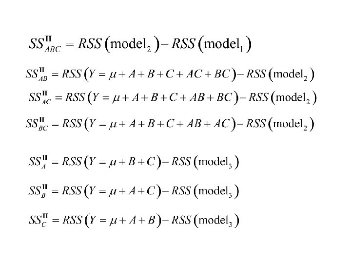
Type II SS • Type two sum of squares are calculated for an effect assuming that the Complete model contains every effect of equal or lesser order. The reduced model has the effect removed ,

The Complete models 1. Y = m + A + B + C + AB + AC + BC + ABC (the three factor model) 2. Y = m + A+ B + C + AB + AC + BC (the all two factor model) 3. Y = m + A + B + C (the all main effects model) The Reduced models For a k-factor effect the reduced model is the all k-factor model with the effect removed

Type III SS • The type III sum of squares is calculated by comparing the full model, to the full model without the effect.

Comments • When using The type I sum of squares the effects are tested in a specified sequence resulting in a increasingly simpler model. The test is valid only the null Hypothesis (H 0) has been accepted in the previous tests. • When using The type II sum of squares the test for a k-factor effect is valid only the all kfactor model can be assumed. • When using The type III sum of squares the tests require neither of these assumptions.

An additional Comment • When the completely randomized design is balanced (equal number of observations per treatment combination) then type I sum of squares, type II sum of squares and type III sum of squares are equal.

Example • A two factor (A and B) experiment, response variable y. • The SPSS data file

Using ANOVA SPSS package Select the type of SS using model

ANOVA table – type I S. S

ANOVA table – type II S. S

ANOVA table – type III S. S

Next Topic Other Experimental Designs