Factorial Experiments Analysis of Variance Experimental Design Dependent

Factorial Experiments Analysis of Variance Experimental Design

• Dependent variable Y • k Categorical independent variables A, B, C, … (the Factors) • Let – a = the number of categories of A – b = the number of categories of B – c = the number of categories of C – etc.

The Completely Randomized Design • We form the set of all treatment combinations – the set of all combinations of the k factors • Total number of treatment combinations – t = abc…. • In the completely randomized design n experimental units (test animals , test plots, etc. are randomly assigned to each treatment combination. – Total number of experimental units N = nt=nabc. .

The treatment combinations can thought to be arranged in a k-dimensional rectangular block 1 1 2 A a 2 B b

C B A

Another way of representing the treatment combinations in a factorial experiment C B . . . A . . . D

Example In this example we are examining the effect of The level of protein A (High or Low) and The source of protein B (Beef, Cereal, or Pork) on weight gains Y (grams) in rats. We have n = 10 test animals randomly assigned to k = 6 diets

The k = 6 diets are the 6 = 3× 2 Level-Source combinations 1. High - Beef 2. High - Cereal 3. High - Pork 4. Low - Beef 5. Low - Cereal 6. Low - Pork

Table Gains in weight (grams) for rats under six diets differing in level of protein (High or Low) and s ource of protein (Beef, Cereal, or Pork) Level of Protein High Protein Low protein Source of Protein Beef Cereal Pork Diet 1 2 3 4 5 6 73 98 94 90 107 49 102 74 79 76 95 82 118 56 96 90 97 73 104 111 98 64 80 86 81 95 102 86 98 81 107 88 102 51 74 97 100 82 108 72 74 106 87 77 91 90 67 70 117 86 120 95 89 61 111 92 105 78 58 82 Mean 100. 0 85. 9 99. 5 79. 2 83. 9 78. 7 Std. Dev. 15. 14 15. 02 10. 92 13. 89 15. 71 16. 55

Example – Four factor experiment Four factors are studied for their effect on Y (luster of paint film). The four factors are: 1) Film Thickness - (1 or 2 mils) 2) Drying conditions (Regular or Special) 3) Length of wash (10, 30, 40 or 60 Minutes), and 4) Temperature of wash (92 ˚C or 100 ˚C) Two observations of film luster (Y) are taken for each treatment combination

The data is tabulated below: Regular Dry Minutes 92 C 1 -mil Thickness 20 3. 4 30 4. 1 40 4. 9 4. 2 60 5. 0 4. 9 2 -mil Thickness 20 5. 5 3. 7 30 5. 7 6. 1 40 5. 5 5. 6 60 7. 2 6. 0 100 C 92 C Special Dry 100 C 19. 6 17. 5 17. 6 20. 9 14. 5 17. 0 15. 2 17. 1 2. 1 4. 0 5. 1 8. 3 3. 8 4. 6 3. 3 4. 3 17. 2 13. 5 16. 0 17. 5 13. 4 14. 3 17. 8 13. 9 26. 6 31. 6 30. 5 29. 5 30. 2 4. 5 5. 9 5. 5 5. 8 25. 6 29. 2 32. 6 22. 5 29. 8 27. 4 31. 4 29. 6 8. 0 9. 9 33. 5 29. 5

Notation Let the single observations be denoted by a single letter and a number of subscripts yijk…. . l The number of subscripts is equal to: (the number of factors) + 1 1 st subscript = level of first factor 2 nd subscript = level of 2 nd factor … Last subsrcript denotes different observations on the same treatment combination

Notation for Means When averaging over one or several subscripts we put a “bar” above the letter and replace the subscripts by • Example: y 241 • •

Profile of a Factor Plot of observations means vs. levels of the factor. The levels of the other factors may be held constant or we may average over the other levels

Definition: A factor is said to not affect the response if the profile of the factor is horizontal for all combinations of levels of the other factors: No change in the response when you change the levels of the factor (true for all combinations of levels of the other factors) Otherwise the factor is said to affect the response:

Definition: • Two (or more) factors are said to interact if changes in the response when you change the level of one factor depend on the level(s) of the other factor(s). • Profiles of the factor for different levels of the other factor(s) are not parallel • Otherwise the factors are said to be additive . • Profiles of the factor for different levels of the other factor(s) are parallel.

• If two (or more) factors interact each factor effects the response. • If two (or more) factors are additive it still remains to be determined if the factors affect the response • In factorial experiments we are interested in determining – which factors effect the response and – which groups of factors interact.

Factor A has no effect B A

Additive Factors B A

Interacting Factors B A

The testing in factorial experiments 1. Test first the higher order interactions. 2. If an interaction is present there is no need to test lower order interactions or main effects involving those factors. All factors in the interaction affect the response and they interact 3. The testing continues with for lower order interactions and main effects for factors which have not yet been determined to affect the response.

Example: Diet Example Summary Table of Cell means Source of Protein Level of Protein Beef High 100. 00 Low 79. 20 Overall 89. 60 Cereal 85. 90 83. 90 84. 90 Pork Overall 99. 50 95. 13 78. 70 80. 60 89. 10 87. 87

Profiles of Weight Gain for Source and Level of Protein

Profiles of Weight Gain for Source and Level of Protein

Models for factorial Experiments Single Factor: A – a levels Random error – Normal, mean 0, std-dev. yij = m + ai + eij Overall mean i = 1, 2, . . . , a; j = 1, 2, . . . , n Effect on y of factor A when A = i

1 observations Levels of A 2 3 a y 11 y 12 y 13 y 21 y 22 y 23 y 31 y 32 y 33 ya 1 ya 2 ya 3 y 1 n y 2 n y 3 n yan m 1 m 2 Normal dist’n Mean of observations Definitions m + a 1 m + a 2 m 3 m + a 3 ma m + aa

Two Factor: A (a levels), B (b levels yijk = m + ai + bj+ (ab)ij + eijk i = 1, 2, . . . , a ; j = 1, 2, . . . , b ; k = 1, 2, . . . , n Overall mean Main effect of A Main effect of B Interaction effect of A and B

Table of Means

Table of Effects – Overall mean, Main effects, Interaction Effects

Three Factor: A (a levels), B (b levels), C (c levels) yijkl = m + ai + bj+ (ab)ij + gk + (ag)ik + (bg)jk+ (abg)ijk + eijkl = m + ai + bj+ gk + (ab)ij + (ag)ik + (bg)jk + (abg)ijk + eijkl Main Two effects factor Three factor Random Interaction error ons i = 1, 2, . . . , a ; j = 1, 2, . . . , b ; k = 1, 2, . . . , c; l = 1, 2, . . . , n

mijk = the mean of y when A = i, B = j, C = k = m + ai + bj+ gk + (ab)ij + (ag)ik + (bg)jk + (abg)ijk Two factor Overall mean Main effects Three factor Interactions i = 1, 2, . . . , a ; j = 1, 2, . . . , b ; k = 1, 2, . . . , c; l = 1, 2, . . . , n

No interaction Levels of C Leve ls of B Levels of A

A, B interact, No interaction with C Levels of C Leve ls of B Levels of A

A, B, C interact Levels of C Leve ls of B Levels of A

Four Factor: yijklm = m + ai + bj+ (ab)ij + gk + (ag)ik + (bg)jk+ (abg)ijk + dl+ (ad)il + (bd)jl+ (abd)ijl + (gd)kl + (agd)ikl + (bgd)jkl+ (abgd)ijkl + eijklm Overall mean =m Two factor Main effects + a i + b j + gk + dl Interactions + (ab)ij + (ag)ik + (bg)jk + (ad)il + (bd)jl+ (gd)kl +(abg)ijk+ (abd)ijl + (agd)ikl + (bgd)jkl Three factor Interactions + (abgd)ijkl + eijklm Four factor Interaction Random error i = 1, 2, . . . , a ; j = 1, 2, . . . , b ; k = 1, 2, . . . , c; l = 1, 2, . . . , d; m = 1, 2, . . . , n where 0 = S ai = S bj= S (ab)ij = S gk = S (ag)ik = S(bg)jk= S (abg)ijk = S dl= S (ad)il = S (bd)jl = S (abd)ijl = S (gd)kl = S (agd)ikl = S (bgd)jkl = S (abgd)ijkl and S denotes the summation over any of the subscripts.

Estimation of Main Effects and Interactions • Estimator of Main effect of a Factor = Mean at level i of the factor - Overall Mean • Estimator of k-factor interaction effect at a combination of levels of the k factors = Mean at the combination of levels of the k factors - sum of all means at k-1 combinations of levels of the k factors +sum of all means at k-2 combinations of levels of the k factors - etc.

Example: • The main effect of factor B at level j in a four factor (A, B, C and D) experiment is estimated by: • The two-factor interaction effect between factors B and C when B is at level j and C is at level k is estimated by:

• The three-factor interaction effect between factors B, C and D when B is at level j, C is at level k and D is at level l is estimated by: • Finally the four-factor interaction effect between factors A, B, C and when A is at level i, B is at level j, C is at level k and D is at level l is estimated by:

Anova Table entries • Sum of squares interaction (or main) effects being tested = (product of sample size and levels of factors not included in the interaction) × (Sum of squares of effects being tested) • Degrees of freedom = df = product of (number of levels - 1) of factors included in the interaction.

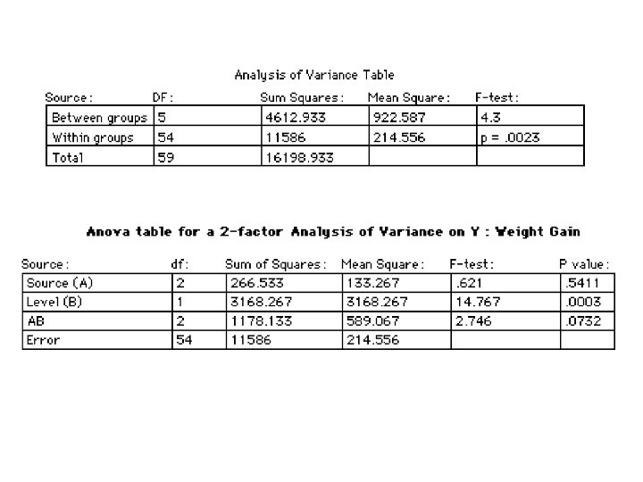
Analysis of Variance (ANOVA) Table Entries (Two factors – A and B)

The ANOVA Table

Analysis of Variance (ANOVA) Table Entries (Three factors – A, B and C)

The ANOVA Table

• The Completely Randomized Design is called balanced • If the number of observations per treatment combination is unequal the design is called unbalanced. (resulting mathematically more complex analysis and computations) • If for some of the treatment combinations there are no observations the design is called incomplete. (some of the parameters - main effects and interactions - cannot be estimated. )

Example: Diet example Mean = 87. 867

Main Effects for Factor A (Source of Protein) Beef 1. 733 Cereal -2. 967 Pork 1. 233

Main Effects for Factor B (Level of Protein) High 7. 267 Low -7. 267

AB Interaction Effects Source of Protein Beef Cereal Pork Level High 3. 133 -6. 267 3. 133 of Protein Low -3. 133 6. 267 -3. 133

Example 2 Paint Luster Experiment

Table: Means and Cell Frequencies

Means and Frequencies for the AB Interaction (Temp - Drying)

Profiles showing Temp-Dry Interaction

Means and Frequencies for the AD Interaction (Temp- Thickness)

Profiles showing Temp-Thickness Interaction

The Main Effect of C (Length)

The Randomized Block Design

• Suppose a researcher is interested in how several treatments affect a continuous response variable (Y). • The treatments may be the levels of a single factor or they may be the combinations of levels of several factors. • Suppose we have available to us a total of N = nt experimental units to which we are going to apply the different treatments.

The Completely Randomized (CR) design randomly divides the experimental units into t groups of size n and randomly assigns a treatment to each group.

The Randomized Block Design • divides the group of experimental units into n homogeneous groups of size t. • These homogeneous groups are called blocks. • The treatments are then randomly assigned to the experimental units in each block - one treatment to a unit in each block.

Experimental Designs • In many experiments were are interested in comparing a number of treatments. (the treatments maybe combinations of levels of several factors. ) • The objective of Experimental design is to reduce the magnitude of random error resulting in more powerful tests to detect experimental effects

The Completely Randomizes Design 1 2 Treats 3 … t Experimental units randomly assigned to treatments

Randomized Block Design Blocks All treats appear once in each block

The Model for a randomized Block Experiment i = 1, 2, …, t j = 1, 2, …, b yij = the observation in the jth block receiving the ith treatment m = overall mean ti = the effect of the ith treatment bj = the effect of the jth Block eij = random error

The Anova Table for a randomized Block Experiment Source S. S. d. f. M. S. F Treat Block Error SST SSB SSE t-1 n-1 (t-1)(b-1) MST MSB MSE MST /MSE MSB /MSE p-value

• A randomized block experiment is assumed to be a two-factor experiment. • The factors are blocks and treatments. • The is one observation per cell. It is assumed that there is no interaction between blocks and treatments. • The degrees of freedom for the interaction is used to estimate error.

Experimental Designs • In many experiments were are interested in comparing a number of treatments. (the treatments maybe combinations of levels of several factors. ) • The objective of Experimental design is to reduce the magnitude of random error resulting in more powerful tests to detect experimental effects

The Completely Randomized Design 1 2 Treats 3 … t Experimental units randomly assigned to treatments

Randomized Block Design Blocks All treats appear once in each block

The matched pair design an experimental design for comparing two treatments Pairs The matched pair design is a randomized block design for t = 2 treatments

The Model for a randomized Block Experiment i = 1, 2, …, t j = 1, 2, …, b yij = the observation in the jth block receiving the ith treatment m = overall mean ti = the effect of the ith treatment bj = the effect of the jth Block eij = random error

The Anova Table for a randomized Block Experiment Source S. S. d. f. M. S. F Treat Block Error SST SSB SSE t-1 n-1 (t-1)(b-1) MST MSB MSE MST /MSE MSB /MSE p-value

Incomplete Block Designs

Randomized Block Design • We want to compare t treatments • Group the N = bt experimental units into b homogeneous blocks of size t. • In each block we randomly assign the t treatments to the t experimental units in each block. • The ability to detect treatment to treatment differences is dependent on the within block variability.

Comments • The within block variability generally increases with block size. • The larger the block size the larger the within block variability. • For a larger number of treatments, t, it may not be appropriate or feasible to require the block size, k, to be equal to the number of treatments. • If the block size, k, is less than the number of treatments (k < t)then all treatments can not appear in each block. The design is called an Incomplete Block Design.

Comments regarding Incomplete block designs • When two treatments appear together in the same block it is possible to estimate the difference in treatments effects. • The treatment difference is estimable. • If two treatments do not appear together in the same block it not be possible to estimate the difference in treatments effects. • The treatment difference may not be estimable.

Example • Consider the block design with 6 treatments and 6 blocks of size two. 1 2 1 4 5 4 2 3 3 5 6 6 • The treatments differences (1 vs 2, 1 vs 3, 2 vs 3, 4 vs 5, 4 vs 6, 5 vs 6) are estimable. • If one of the treatments is in the group {1, 2, 3} and the other treatment is in the group {4, 5, 6}, the treatment difference is not estimable.

Definitions • Two treatments i and i* are said to be connected if there is a sequence of treatments i 0 = i, i 1, i 2, … i. M = i* such that each successive pair of treatments (ij and ij+1) appear in the same block • In this case the treatment difference is estimable. • An incomplete design is said to be connected if all treatment pairs i and i* are connected. • In this case all treatment differences are estimable.

Example • Consider the block design with 5 treatments and 5 blocks of size two. 1 2 1 4 1 2 3 3 5 4 • This incomplete block design is connected. • All treatment differences are estimable. • Some treatment differences are estimated with a higher precision than others.

Definition An incomplete design is said to be a Balanced Incomplete Block Design. 1. if all treatments appear in exactly r blocks. • This ensures that each treatment is estimated with the same precision 2. if all treatment pairs i and i* appear together in exactly l blocks. • This ensures that each treatment difference is estimated with the same precision. • The value of l is the same for each treatment pair.

Some Identities Let b = the number of blocks. t = the number of treatments k = the block size r = the number of times a treatment appears in the experiment. l = the number of times a pair of treatment appears together in the same block 1. bk = rt • Both sides of this equation are found by counting the total number of experimental units in the experiment. 2. r(k-1) = l (t – 1) • Both sides of this equation are found by counting the total number of experimental units that appear with a specific treatment in the experiment.

BIB Design A Balanced Incomplete Block Design (b = 15, k = 4, t = 6, r = 10, l = 6)

An Example A food processing company is interested in comparing the taste of six new brands (A, B, C, D, E and F) of cereal. For this purpose: • subjects will be asked to taste and compare these cereals scoring them on a scale of 0 - 100. • For practical reasons it is decided that each subject should be asked to taste and compare at most four of the six cereals. • For this reason it is decided to use b = 15 subjects and a balanced incomplete block design to assess the differences in taste of the six brands of cereal.

The design and the data is tabulated below:

Analysis of Block Experiments

Analysis of Block Experiments The purpose of such experiments is to estimate the effects of treatments applied to some material (experimental units, subjects etc. ) grouped into relatively homogeneous groups (blocks). The variability within the groups (blocks) will be considerably less than if the subjects were left ungrouped. This will lead to a more powerful analysis for comparing the treatments.

The basic model for block experiments Suppose we have t treatments and b blocks of size k. The Assumption of Additivity

Let if treat n is applied to mth unit in jth block otherwise

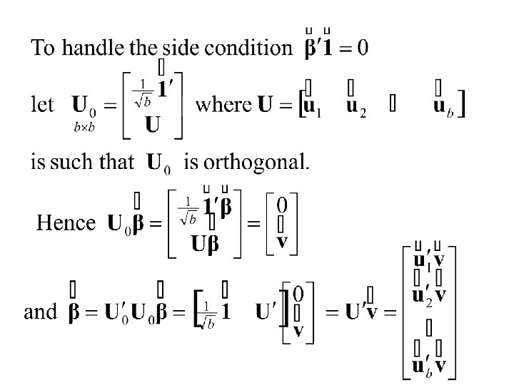
Not of full rank

Now define the incidence matrix

Note Now if treat n is applied to mth unit in jth block otherwise

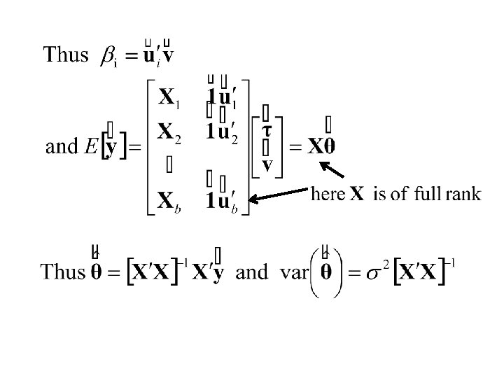
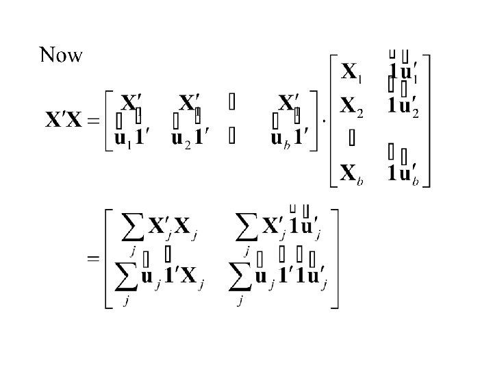
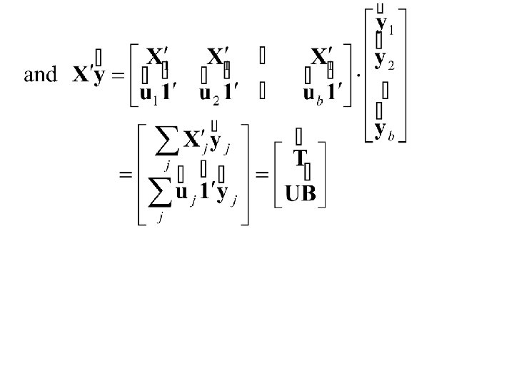
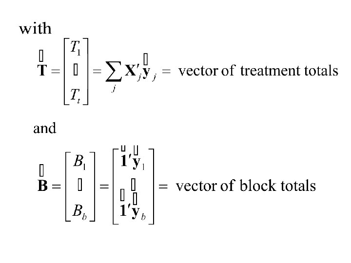
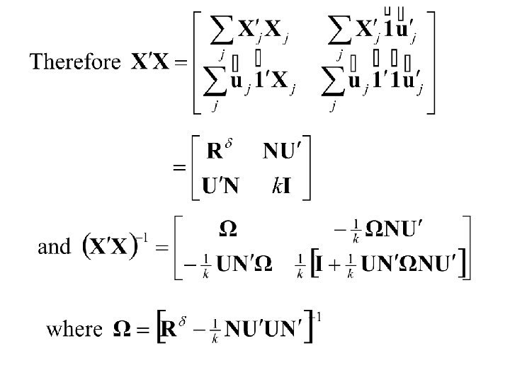
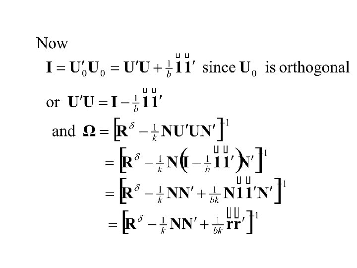
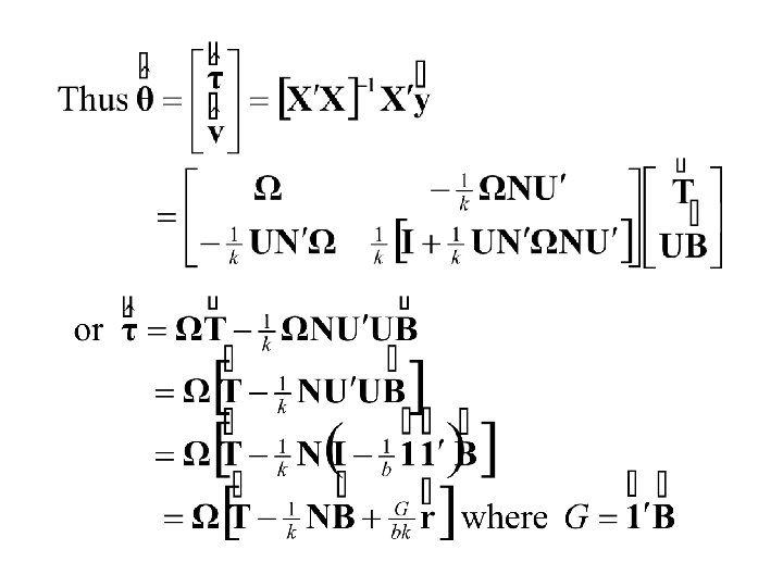
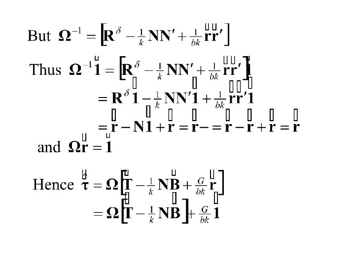
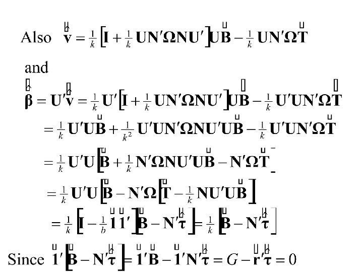
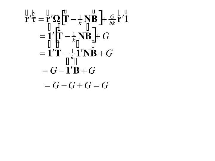
Thus Also and

Thus and

Finally

Summary: The Least Squares Estimates The Residual Sum of Squares

Hence

Summary: The Least Squares Estimates The Residual Sum of Squares