Factor analysis Caroline van Baal March 3 rd

Factor analysis Caroline van Baal March 3 rd 2004, Boulder

Phenotypic Factor Analysis • (Approximate) description of the relations between different variables – Compare to Cholesky decomposition • Testing of hypotheses on relations between different variables by comparing different (nested) models – How many underlying factors?

Factor analysis and related methods • Data reduction – Consider 6 variables: – Height, weight, arm length, leg length, verbal IQ, performal IQ – You expect the first 4 to be correlated, and the last 2 to be correlated, but do you expect high correlations between the first 4 and the last 2?

Data analysis in nonexperimental designs using latent constructs • • • Principal Components Analysis Triangular Decomposition (Cholesky) Exploratory Factor Analysis Confirmatory Factor Analysis Structural Equation Models

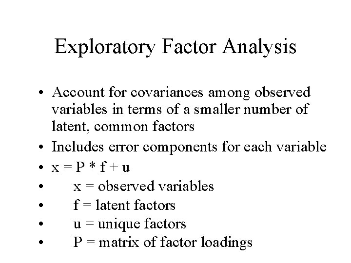
Exploratory Factor Analysis • Account for covariances among observed variables in terms of a smaller number of latent, common factors • Includes error components for each variable • x=P*f+u • x = observed variables • f = latent factors • u = unique factors • P = matrix of factor loadings

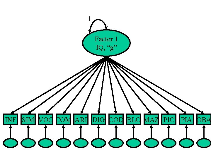
1 Factor 1 IQ, “g” INF SIM VOC COM ARI DIG COD BLC MAZ PIC PIA OBA

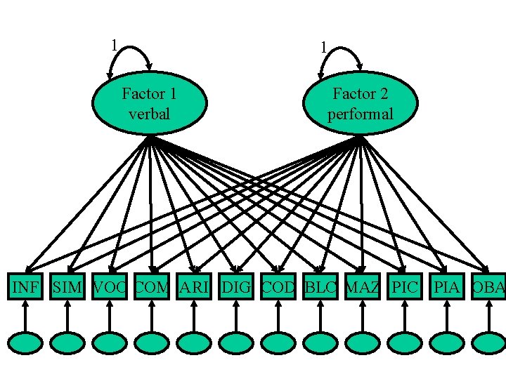
1 1 Factor 1 verbal Factor 2 performal INF SIM VOC COM ARI DIG COD BLC MAZ PIC PIA OBA

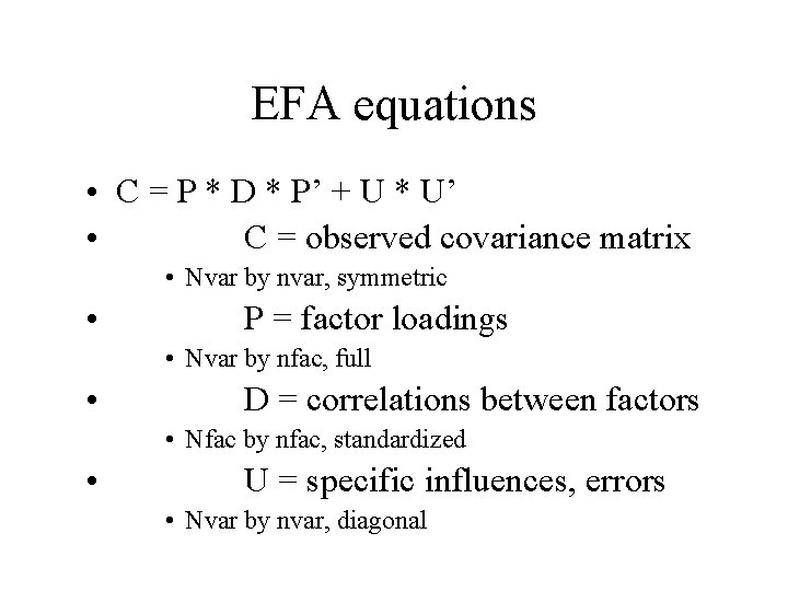
EFA equations • C = P * D * P’ + U * U’ • C = observed covariance matrix • Nvar by nvar, symmetric • P = factor loadings • Nvar by nfac, full • D = correlations between factors • Nfac by nfac, standardized • U = specific influences, errors • Nvar by nvar, diagonal

Exploratory factor analysis • No prior assumption on number of factors • All variables load on all latent factors • Factors are either all correlated or all uncorrelated • Unique factors are uncorrelated • Underidentification

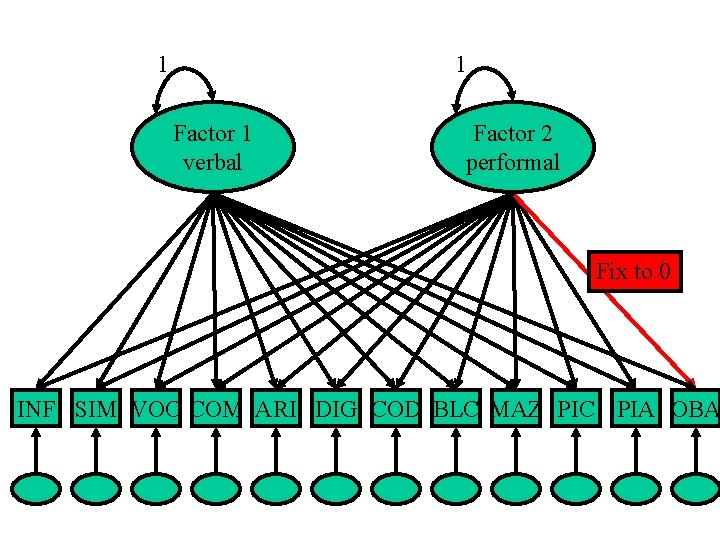
1 1 Factor 1 verbal Factor 2 performal Fix to 0 INF SIM VOC COM ARI DIG COD BLC MAZ PIC PIA OBA

Confirmatory factor analysis • An initial model is constructed, because: – its elements are described by a theoretical process – its elements have been obtained from a previous analysis in another sample • • The model has a specific number of factors Variables do not have to load on all factors Measurement errors may correlate Some latent factors may be correlated, while others are not

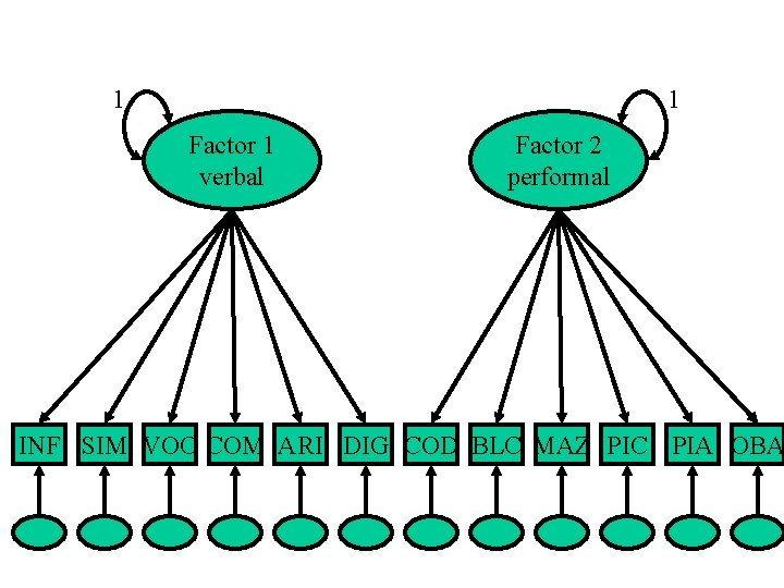
1 1 Factor 1 verbal Factor 2 performal INF SIM VOC COM ARI DIG COD BLC MAZ PIC PIA OBA

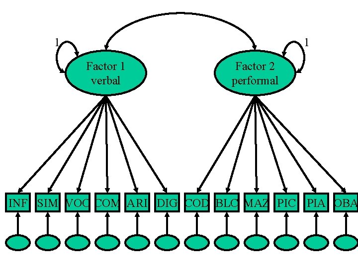
1 1 Factor 1 verbal Factor 2 performal INF SIM VOC COM ARI DIG COD BLC MAZ PIC PIA OBA

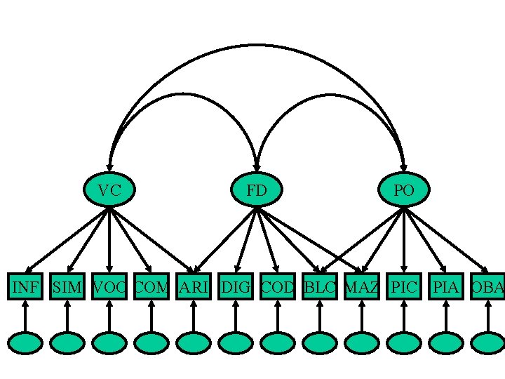
VC FD PO INF SIM VOC COM ARI DIG COD BLC MAZ PIC PIA OBA

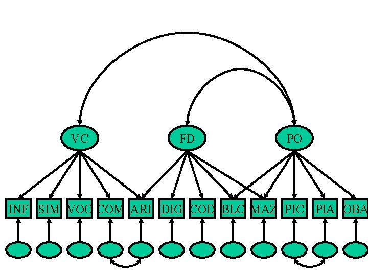
VC FD PO INF SIM VOC COM ARI DIG COD BLC MAZ PIC PIA OBA

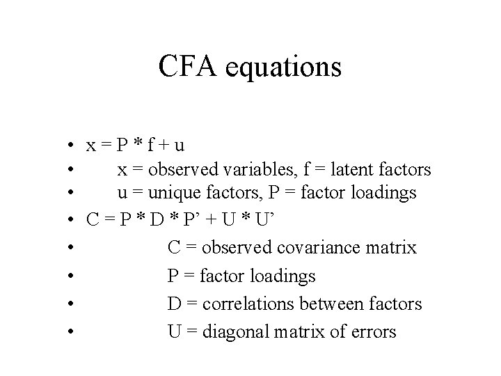
CFA equations • x=P*f+u • x = observed variables, f = latent factors • u = unique factors, P = factor loadings • C = P * D * P’ + U * U’ • C = observed covariance matrix • P = factor loadings • D = correlations between factors • U = diagonal matrix of errors

Structural equations models • The factor model x = P * f + u is sometimes referred to as the measurement model • The relations between latent factors can also be modeled • This is done in the covariance structure model, or the structural equations model • Higher order factor models

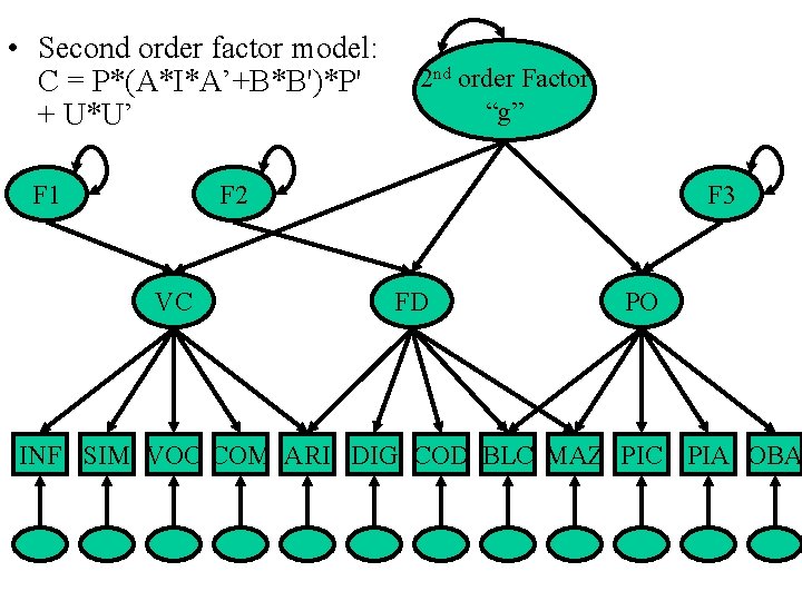
• Second order factor model: C = P*(A*I*A’+B*B')*P' + U*U’ F 1 2 nd order Factor “g” F 2 VC F 3 FD PO INF SIM VOC COM ARI DIG COD BLC MAZ PIC PIA OBA

Five steps characterize structural equation models • Model specification • Identification – E. g. , if a factor loads on 2 variables only, multiple solutions are possible, and the factor loadings have to be equated • Estimation of parameters • Testing of goodness of fit • Respecification • K. A. Bollen & J. Scott Long: Testing Structural Equation Models, 1993, Sage Publications

Practice! • IQ and brain volumes (MRI) • 3 brain volumes – Total cerebellum, Grey matter, White matter • 2 IQ subtests – Calculation, Letters / numbers • Brain and IQ factors are correlated • Datafile: mri-IQ-all-twin. A-5. dat

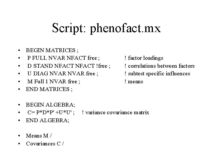
Script: phenofact. mx • BEGIN MATRICES ; • P FULL NVAR NFACT free ; • D STAND NFACT !free ; • U DIAG NVAR free ; • M Full 1 NVAR free ; • END MATRICES ; • BEGIN ALGEBRA; • C= P*D*P' +U*U' ; • END ALGEBRA; • Means M / • Covariances C / ! factor loadings ! correlations between factors ! subtest specific influences ! means ! variance covariance matrix

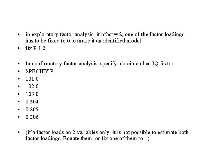
• in exploratory factor analysis, if nfact = 2, one of the factor loadings has to be fixed to 0 to make it an identified model • fix P 1 2 • • In confirmatory factor analysis, specify a brain and an IQ factor SPECIFY P 101 0 102 0 103 0 0 204 0 205 0 206 • (if a factor loads on 2 variables only, it is not possible to estimate both factor loadings. Equate them, or fix one of them to 1)

Phenotypic Correlations: MRI-IQ, Dutch twins (A), n=111/296 pairs brain cereb Cerebellum 1 Grey. 63 White. 61 calculation. 23 Letter/numb. . 30 brain grey brain IQ white calc IQ L/n 1. 55. 25. 19 1. 26. 19 1 1. 46

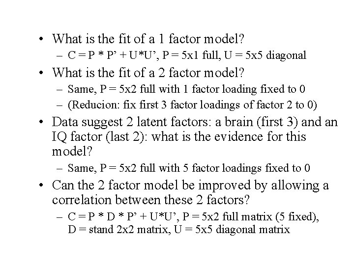
• What is the fit of a 1 factor model? – C = P * P’ + U*U’, P = 5 x 1 full, U = 5 x 5 diagonal • What is the fit of a 2 factor model? – Same, P = 5 x 2 full with 1 factor loading fixed to 0 – (Reducion: fix first 3 factor loadings of factor 2 to 0) • Data suggest 2 latent factors: a brain (first 3) and an IQ factor (last 2): what is the evidence for this model? – Same, P = 5 x 2 full with 5 factor loadings fixed to 0 • Can the 2 factor model be improved by allowing a correlation between these 2 factors? – C = P * D * P’ + U*U’, P = 5 x 2 full matrix (5 fixed), D = stand 2 x 2 matrix, U = 5 x 5 diagonal matrix

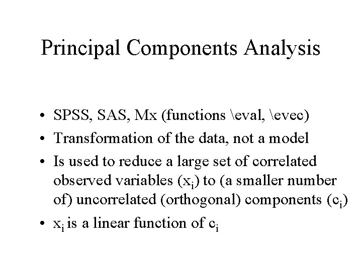
Principal Components Analysis • SPSS, SAS, Mx (functions eval, evec) • Transformation of the data, not a model • Is used to reduce a large set of correlated observed variables (xi) to (a smaller number of) uncorrelated (orthogonal) components (ci) • xi is a linear function of ci

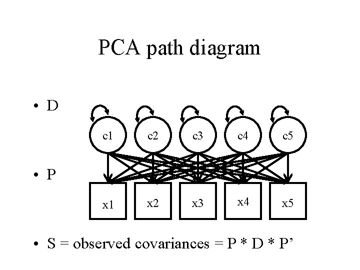
PCA path diagram • D c 1 c 2 c 3 c 4 c 5 x 1 x 2 x 3 x 4 x 5 • P • S = observed covariances = P * D * P’

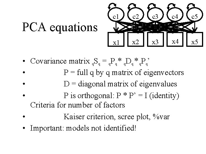
PCA equations c 1 c 2 c 3 c 4 c 5 x 1 x 2 x 3 x 4 x 5 • Covariance matrix q. Sq = q. Pq * q. Dq * q. Pq’ • P = full q by q matrix of eigenvectors • D = diagonal matrix of eigenvalues • P is orthogonal: P * P’ = I (identity) Criteria for number of factors • Kaiser criterion, scree plot, %var • Important: models not identified!

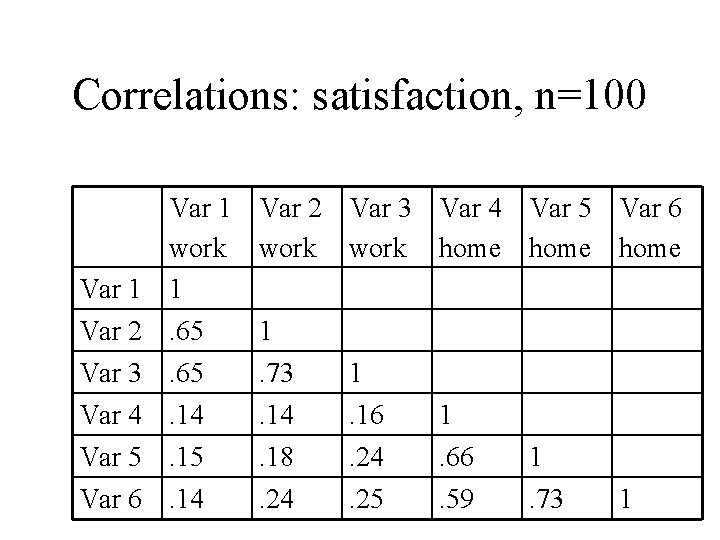
Correlations: satisfaction, n=100 Var 1 Var 2 Var 3 Var 4 Var 5 Var 6 Var 1 work 1. 65. 14. 15. 14 Var 2 Var 3 Var 4 Var 5 Var 6 work home 1. 73. 14. 18. 24 1. 16. 24. 25 1. 66. 59 1. 73 1

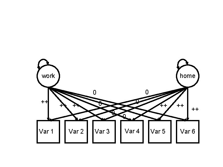
work home 0 0 ++ ++ ++ 0 0 0 Var 1 Var 2 Var 3 ++ ++ ++ 0 Var 4 Var 5 Var 6

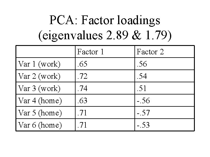
PCA: Factor loadings (eigenvalues 2. 89 & 1. 79) Var 1 (work) Var 2 (work) Factor 1. 65. 72 Factor 2. 56. 54 Var 3 (work) Var 4 (home) Var 5 (home) Var 6 (home) . 74. 63. 71 . 51 -. 56 -. 57 -. 53

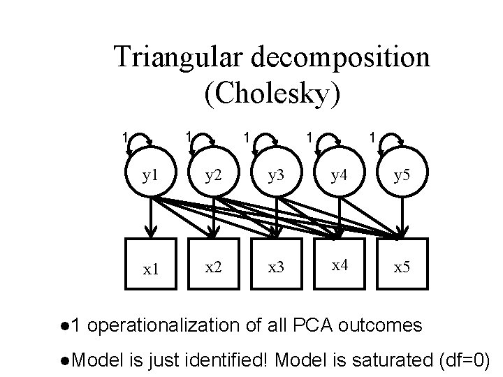
Triangular decomposition (Cholesky) 1 1 l 1 1 y 1 y 2 y 3 y 4 y 5 x 1 x 2 x 3 x 4 x 5 operationalization of all PCA outcomes l. Model is just identified! Model is saturated (df=0)

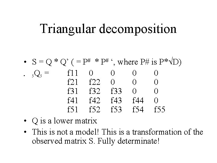
Triangular decomposition • S = Q * Q’ ( = P# * P# ‘, where P# is P* D) f 11 0 0 5 Q 5 = • f 21 f 22 0 0 0 f 31 f 32 f 33 0 0 f 41 f 42 f 43 f 44 0 f 51 f 52 f 53 f 54 f 55 • Q is a lower matrix • This is not a model! This is a transformation of the observed matrix S. Fully determinate!

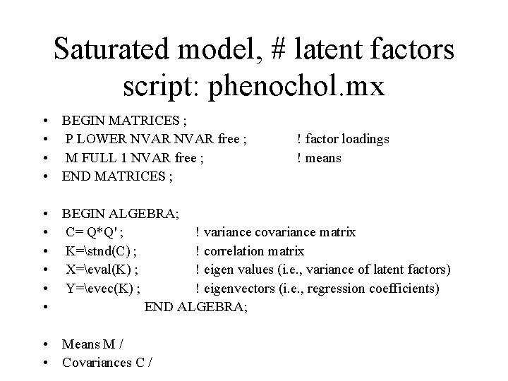
Saturated model, # latent factors script: phenochol. mx • BEGIN MATRICES ; • P LOWER NVAR free ; • M FULL 1 NVAR free ; • END MATRICES ; ! factor loadings ! means • BEGIN ALGEBRA; • C= Q*Q' ; ! variance covariance matrix • K=stnd(C) ; ! correlation matrix • X=eval(K) ; ! eigen values (i. e. , variance of latent factors) • Y=evec(K) ; ! eigenvectors (i. e. , regression coefficients) • END ALGEBRA; • Means M / • Covariances C /