Facility Location Decisions n Classifying location decisions n

Facility Location Decisions n Classifying location decisions n n n Driving force (critical factor - traffic, labor rates, emergency facilities, obnoxious facilities) Number of facilities Discrete vs. continuous choices Data aggregation Time Horizon 1

Facility Location n n Rent Curve - The rent of land is a decreasing function of the distance to the market Weight gaining vs. weight losing industries n n n Weight losing should locate close to raw materials Weight gaining should locate close to market Tapered (concave) transportation costs n n The derivative of total transportation cost is non-increasing with the distance to the market (holds for inbound and outbound costs) Optimal solution will always locate either at raw materials or at market (extreme point solution) 2

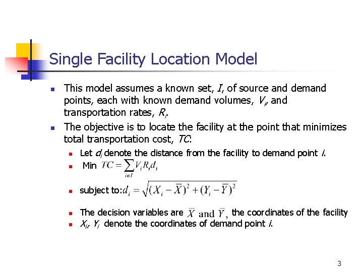
Single Facility Location Model n n This model assumes a known set, I, of source and demand points, each with known demand volumes, Vi, and transportation rates, Ri. The objective is to locate the facility at the point that minimizes total transportation cost, TC: n Let di denote the distance from the facility to demand point i. n n Min subject to: The decision variables are the coordinates of the facility Xi, Yi denote the coordinates of demand point i. 3

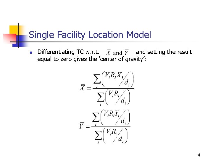
Single Facility Location Model n Differentiating TC w. r. t. and setting the result equal to zero gives the ‘center of gravity’: 4

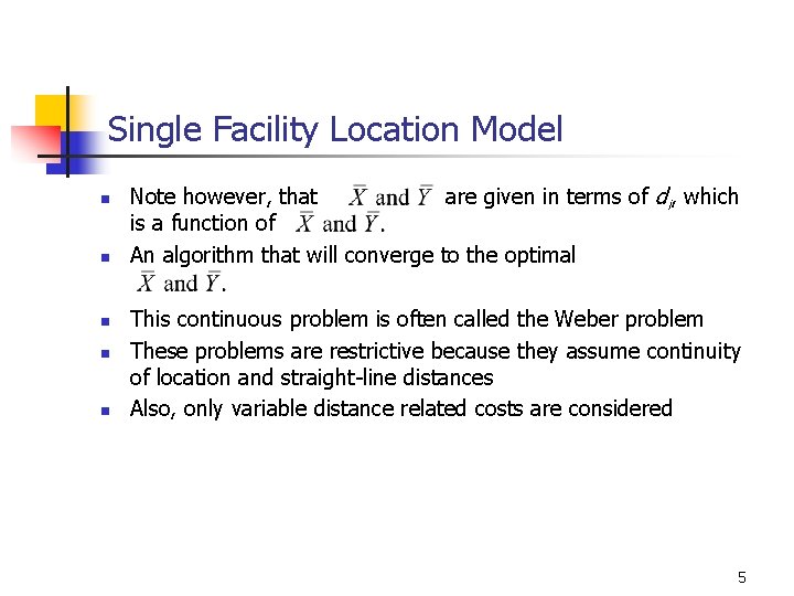
Single Facility Location Model n n n Note however, that are given in terms of di, which is a function of An algorithm that will converge to the optimal This continuous problem is often called the Weber problem These problems are restrictive because they assume continuity of location and straight-line distances Also, only variable distance related costs are considered 5

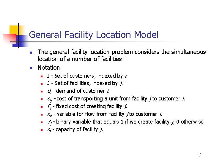
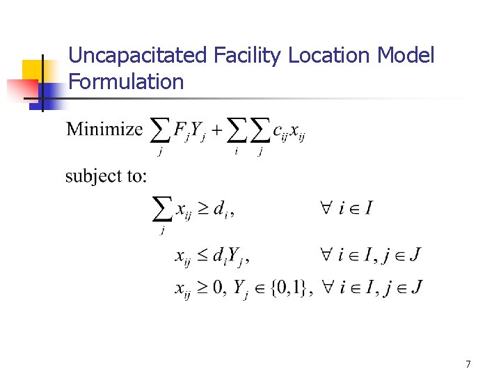
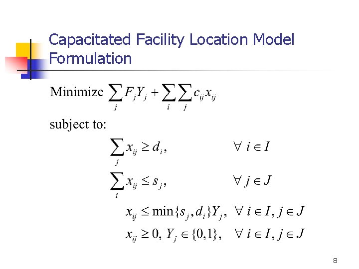
General Facility Location Model n n The general facility location problem considers the simultaneous location of a number of facilities Notation: n I - Set of customers, indexed by i. n J - Set of facilities, indexed by j. n di - demand of customer i. n cij - cost of transporting a unit from facility j to customer i. n Fj - fixed cost of creating facility j. n xij - variable for flow from facility j to customer i. n Yj - binary variable that equals 1 if we create facility j, 0 otherwise n sj - capacity of facility j. 6

Uncapacitated Facility Location Model Formulation 7

Capacitated Facility Location Model Formulation 8

Location Decisions and Risk Pooling n n n Suppose we must serve n independent markets with a single product, and each market has average demand period of D and standard deviation (we neglect lead times for simplicity) Assume we have a service level policy to ensure that the probability of not stocking out in each period equals Suppose we serve each market using a single inventory stocking location. The standard deviation of demand as seen by the single stocking location in each period equals If demand is normally distributed, the safety stock required at the single location equals z 9

Location Decisions and Risk Pooling n n n Suppose, at the other extreme, we place an inventory stocking location in each of the n markets Each stocking location will need to hold z to meet the service level requirement The system-wide safety stock equals z n > z This example illustrates the risk-pooling effects of location decisions The more stocking locations we have, the more duplication in safety stock we have The single location, however, will incur the maximum transportation costs, while n locations should minimize the transportation costs 10

Location Decisions and Risk Pooling n n n The safety stock costs and transportation costs are at odds with each other We need to strike a balance between the two Models for this decision are currently limited (Prof. Shen has worked on a model that addresses this tradeoff) However, this simple analysis can provide strong insights If inventory costs dominate transportation costs (as in expensive computing chips), we are driven to have less stocking points; if transport costs dominate (as in coal), then we are driven to have more stocking locations One thing not included in the analysis is delivery lead time and its impact on service levels – obviously more locations closer to markets can respond much more quickly to customers 11

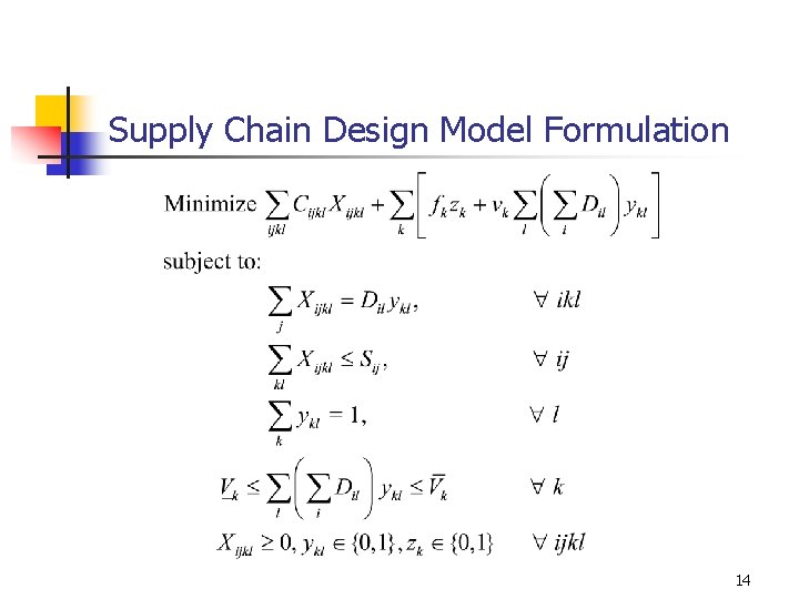
Supply Chain Design Model n n n The objective of this model is to determine the warehouse and plant configuration that minimizes total costs for production and distribution of multiple products. Based on Geoffrion and Graves, 1974, “Multicommodity distribution system design by Benders decomposition, ” Management Science, v 20, n 5. (see Tech. Suppl. , Ch. 13) Notation: n i - index for commodities n j - index for plants n k - index for warehouses n l - index for customer zones 12

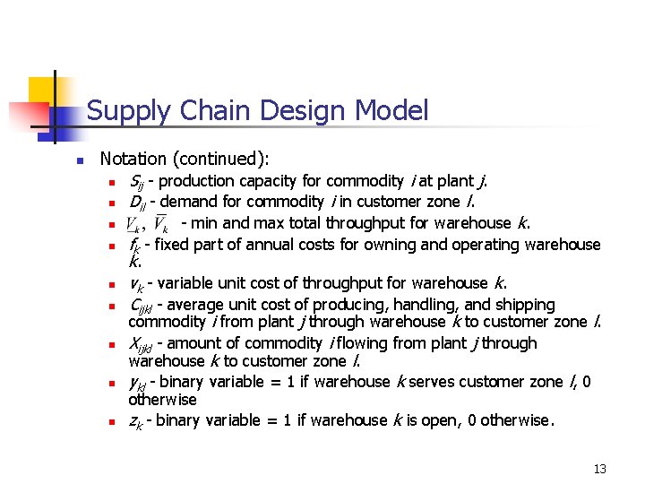
Supply Chain Design Model n Notation (continued): n Sij - production capacity for commodity i at plant j. n Dil - demand for commodity i in customer zone l. n n n n - min and max total throughput for warehouse k. fk - fixed part of annual costs for owning and operating warehouse k. vk - variable unit cost of throughput for warehouse k. Cijkl - average unit cost of producing, handling, and shipping commodity i from plant j through warehouse k to customer zone l. Xijkl - amount of commodity i flowing from plant j through warehouse k to customer zone l. ykl - binary variable = 1 if warehouse k serves customer zone l, 0 otherwise zk - binary variable = 1 if warehouse k is open, 0 otherwise. 13

Supply Chain Design Model Formulation 14

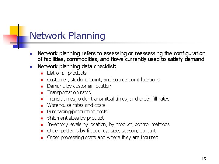
Network Planning n n Network planning refers to assessing or reassessing the configuration of facilities, commodities, and flows currently used to satisfy demand Network planning data checklist: n n n List of all products Customer, stocking point, and source point locations Demand by customer location Transportation rates Transit times, order transmittal times, and order fill rates Warehouse rates and costs Purchasing/production costs Shipment sizes by product Inventory levels by location, by product, control methods Order patterns by frequency, size, season, content Order processing costs and where they are incurred 15

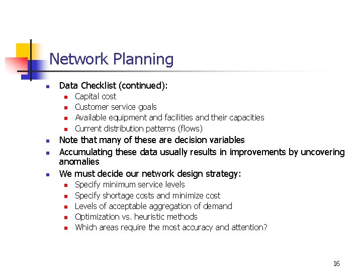
Network Planning n Data Checklist (continued): n n n n Capital cost Customer service goals Available equipment and facilities and their capacities Current distribution patterns (flows) Note that many of these are decision variables Accumulating these data usually results in improvements by uncovering anomalies We must decide our network design strategy: n n n Specify minimum service levels Specify shortage costs and minimize cost Levels of acceptable aggregation of demand Optimization vs. heuristic methods Which areas require the most accuracy and attention? 16