Face Recognition Using the Nearest Feature Line Method

Face Recognition Using the Nearest Feature Line Method Stan Z. Li and Juwei Lu Nearest_feature_line. pdf

Problem • Face recognition – Detect faces – Must account for different viewpoints, illumination, and expression • Which features to use? • How do you classify a new face image?

Geometric Feature Based Methods • Positives: – Data reduction – Insensitive to illumination – Insensitive to viewpoint • Negatives: – Extraction of facial features are unreliable. We win?

Template Matching • Eigenface representation • Face space constructed by – Karhunen-Loeve transform (? ) – Principal Component Analysis • Every face image is a feature point (vector of weights) • Nearest Neighbor Classifier

• “Generalize the representational capacity of available prototype images. ”

Nearest Feature Line (NFL) • Assumption: Every test image has at least 2 distinct features. • Feature line (FL) ~variants of the two images under variations. • Classification using minimum distance between test feature point and FL’s.

The Feature Space • Eigenface space – Training set of N face images T = {z 1, z 2, … z. N}. – Construct covariance matrix: 1/N * sum{n=1, N} (znz)(zn-z)^T, where z is the average of T. – Apply PCA to covariance matrix. – With first N’ eigenvectors, project each training image into the eigenface space by: xn = psi^T(zn-z), where psi is the set of N’ eigenvectors. – Classify a test image by projecting into eigenspace and assigning to nearest class (Nearest Neighbor).

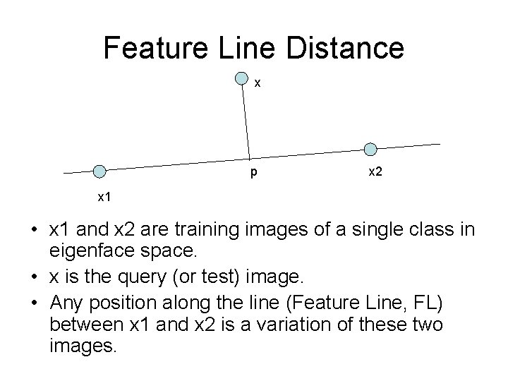
Feature Line Distance x p x 2 x 1 • x 1 and x 2 are training images of a single class in eigenface space. • x is the query (or test) image. • Any position along the line (Feature Line, FL) between x 1 and x 2 is a variation of these two images.

FL Distance cont’d. • Project p onto the x 1, x 2 Feature Line. – – p = x 1 + u(x 2 -x 1) Solve for u u describes the position of p relative to x 1 and x 2 When: • • • u = 0, p = x 1 u = 1, p = x 2 0 < u < 1, p is an interpolating point between x 1 and x 2 u > 1, p is a forward extrapolating point on the x 2 side u < 0, p is a backward extrapolating point on the x 1 side

FL Distance cont’d. • The linear variations on FL provides MANY more feature points. • Variations aren’t linear though. – Use higher order curves – Use splines • However, FL is sufficient for the classification described as follows…. .

NFL- Based Classification • Given a test image, x, assign it to a class in the training set. • For each pair of feature points, calculate the FL distance between it and x. • Sort the distances in ascending order (with class identifier, 2 feature points, and u). • The NFL distance is the first rank distance. • Yields best matched class and two best matched feature points.

Results • See paper.