
Face Detection using the Spectral Histogram representation By
Face Detection using the Spectral Histogram representation By: Christopher Waring, Xiuwen Liu Department of Computer Science Florida State University Presented by: Tal Blum blum+@cs. cmu. edu
Sources • The presentation is based on a few resources by the authors: – Exploration of the Spectral Histogram for Face Detection – M. Sc thesis by Christopher Waring (2002) – Spectral Histogram Based Face Detection – IEEE (2003) – Rotation Invariant Face Detection Using Spectral Histograms & SVM – CVPR submission – Independent Spectral Representation of images for Recognition – Optical Society of America (2003)
Overview • Spectral Histogram – Overview of Gibbs Sampling + Simulated annealing • Method for Lighting Normalization • Data used • 3 Algorithms – SH + Neural Networks – SH + SVM – Rotation Invariant SH +SVM • Experimental Results • Conclusions & Discussions
Two Approaches to Object Detection • Curse of dimensionality – Features should be: (Vasconcelos) • Independent • have low Bayes Error • 2 main Approaches in Object Detection: – Complicated Features with many interactions • • Require many data points Use syntactic variations that mimic the real variations Estimation Error might be high Assuming Model or Parameter structure – Small set of features or small number of values • This is the case for Spectral Histograms • The Bayes Error might be high (Vasconcelos) • Estimation Error is low
Why Spectral Histograms? • Translation Invariant – Therefore insensitive to incorrect alignment. • (surprisingly) seem to be able to separate Objects from Non-Objects well. • Good performance with a very small feature set. • Good performance with a large rotation invariance. • Don’t rely at all on any global spatial information • Combining of variant and invariant features • Will play a more Important role

What is Spectral Histogram
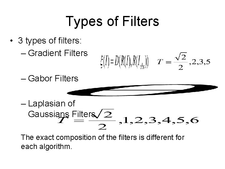
Types of Filters • 3 types of filters: – Gradient Filters – Gabor Filters – Laplasian of Gaussians Filters The exact composition of the filters is different for each algorithm.
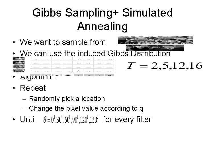
Gibbs Sampling+ Simulated Annealing • We want to sample from • We can use the induced Gibbs Distribution • Algorithm: • Repeat – Randomly pick a location – Change the pixel value according to q • Until for every filter
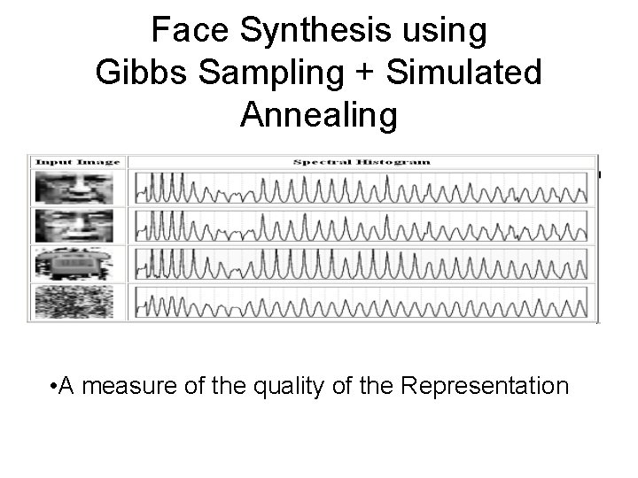
Face Synthesis using Gibbs Sampling + Simulated Annealing • A measure of the quality of the Representation
Comparison - PCA vs. Spectral Histogram Original Image Reconstructed Images
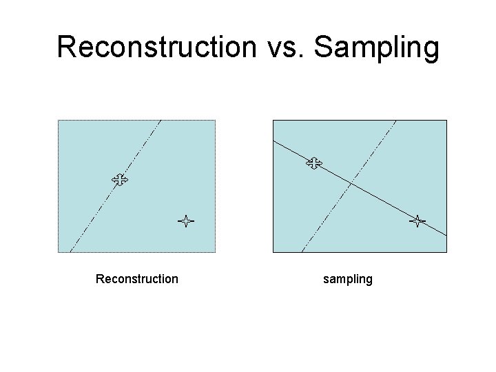
Reconstruction vs. Sampling Reconstruction sampling
Spectral Histograms of several images
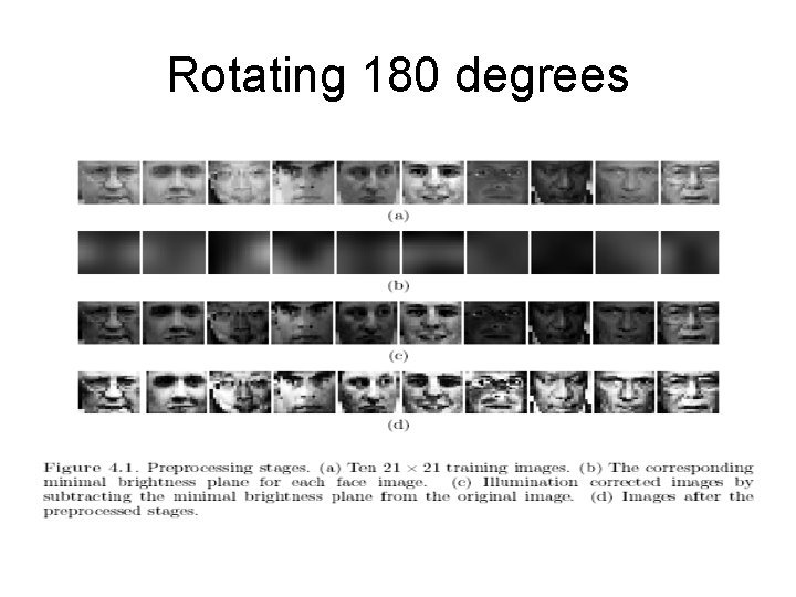
Lighting correction • They use a 21 x 21 sized images • Minimal brightness plane of 3 x 3 is computed from each 7 x 7 block • A 21 x 21 correction plane is computed by bi-linear interpolation • Histogram Normalization is applied
Lighting correction
Detection & Post Processing • Detection is don on 3 scaled Gaussian pyramid, each scale down sampled by 1. 1 • detections within 3 pixels are merged • A detection is marked as final if it is found at at least two concurrent levels • A detection counts as correct if at least half of the face lies within the detection window
Adaptive Threshold
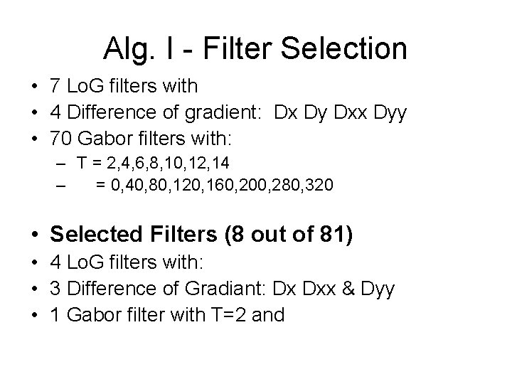
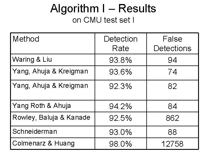
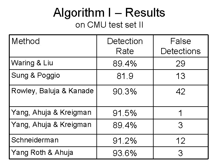
Algorithm I using a Neural Network • Neural Network was used as a classifier – Training with back propagation • Data Processing – 1500 Face images & 8000 Non-Face images – Bootstrapping was used to limit the # non faces (Sung Poggio) leaving 800 Non-Faces • Use 8 filters with 80 bins in each
Alg. I - Filter Selection • 7 Lo. G filters with • 4 Difference of gradient: Dx Dy Dxx Dyy • 70 Gabor filters with: – T = 2, 4, 6, 8, 10, 12, 14 – = 0, 40, 80, 120, 160, 200, 280, 320 • Selected Filters (8 out of 81) • 4 Lo. G filters with: • 3 Difference of Gradiant: Dx Dxx & Dyy • 1 Gabor filter with T=2 and
Spectral Histograms of several images
Algorithm I – Results on CMU test set I Method Yang, Ahuja & Kreigman Detection Rate 93. 8% 93. 6% False Detections 94 74 Yang, Ahuja & Kreigman 92. 3% 82 Yang Roth & Ahuja 94. 2% 92. 5% 84 862 93. 0% 98. 0% 88 12758 Waring & Liu Rowley, Baluja & Kanade Schneiderman Colmenarz & Huang
Algorithm I – Results on CMU test set II Method Detection Rate 89. 4% 81. 9 False Detections 29 13 Rowley, Baluja & Kanade 90. 3% 42 Yang, Ahuja & Kreigman 91. 5% 89. 4% 1 3 91. 2% 93. 6% 12 3 Waring & Liu Sung & Poggio Yang, Ahuja & Kreigman Schneiderman Yang Roth & Ahuja
Algorithm II using a SVM • SVM instead of a Neural Network • They use more filters – 34 filters (instead of 7) – 359 bins (instead of 80) • 4500 randomly rotated Face images & 8000 Non-Face images from before
Algorithm II (SVM) Filters • The filters were hand picked • Filters: – The Intensity filter – 4 Difference of Gradient filters Dx, Dy, Dxx &Dyy – 5 Lo. G filgers – 24 gabor filters with • Local & Global Constraints • Using Histograms as features
Spectral Histograms of several images
Algorithm II (SVM) Results
Old Results






Algorithm III using SVM + rotation invariant features • Same features as in Alg. II • The Features enable 180 degrees of rotation invariance • Rotate the image 180 degrees and switch Histograms achieving 360 degrees invariance
Rotating 180 degrees
Combining the two classifiers
Results Upright test sets
Results Rotated test sets


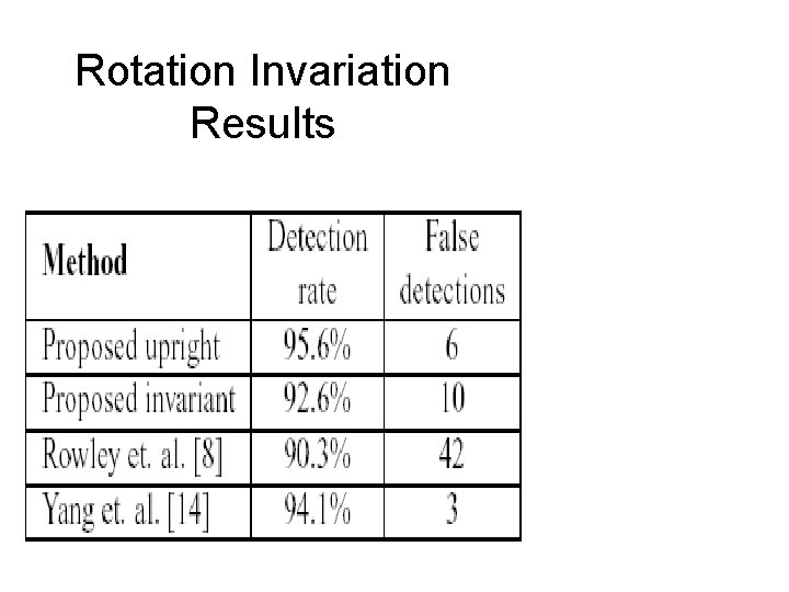
Rotation Invariation Results

More pictures


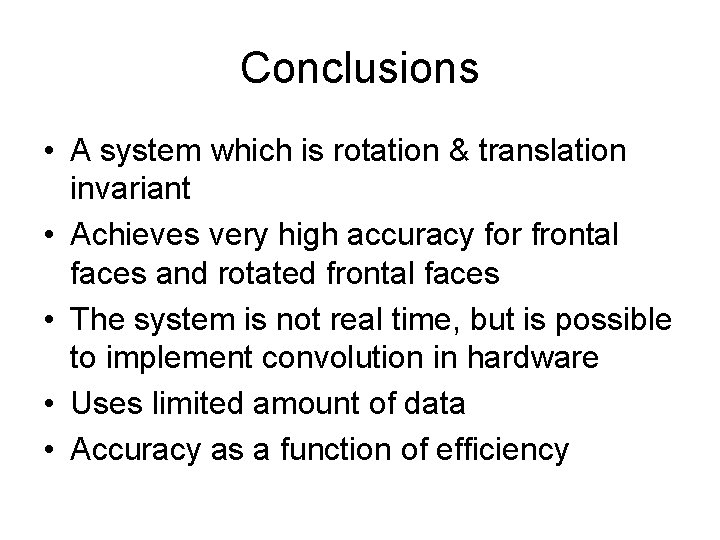
Conclusions • A system which is rotation & translation invariant • Achieves very high accuracy for frontal faces and rotated frontal faces • The system is not real time, but is possible to implement convolution in hardware • Uses limited amount of data • Accuracy as a function of efficiency
Conclusions (2) • Faces are identifiable through local spatial dependencies where the global ones can be globally modeled as histograms • The problem with spatial methods is the estimation of the parameters • The SH representation is independent of classifier choice • SVM outperforms Neural Networks • The Problems and the Errors of this system are considerably different than of other systems
Conclusions (3) • Localization in Space and Scale is not as good as other methods • Translation Invariant features can enable a coarser sampling the image • Use adaptive thresholding • Use several scales to improve performance • SH can be used for sampling of objects
- Slides: 46