Eyewall replacement cycles and the tropical cyclone boundary

Eyewall replacement cycles and the tropical cyclone boundary layer Jeffrey D. Kepert High Impact Weather Bureau of Meteorology Research and Development

Eyewall contraction, intensification and replacement max tangential acceleration Willoughby, 1988, AMM

How do secondary eyewalls form? Nobody really knows … not for sure, anyway • i. e. there is no consensus Numerous explanations, some have gone, others remain • Vortex Rossby Waves • Beta-skirt axisymmetrisation • WISHE • Environmental influences • Boundary-layer supergradient flow • and more …

What is the role of the BL in an ERC? Goal: Investigate the boundary-layer flow in a cyclone with concentric eyewalls Method: Diagnostic models of the tropical cyclone boundary layer • Model the BL flow as the response to an imposed, axisymmetric pressure field that represents the rest of the cyclone • One part of a two-way interaction: the cyclone structure and intensity affects the BL flow, but not vice versa. • Enables controlled experiments Three models: • Kepert and Wang (2001): Full nonlinear equations, realistic physics, numerical solution. • Kepert (2001): Linearised equations, simplified physics, analytical solution. • Ooyama (1969) and Emanuel (1986): Simplified depth-averaged equations, analytical solution.

Model description • Aim: controlled experiments on boundary-layer flow • Control => hold rest of the cyclone fixed • Prescribe p at top of model, solve equations within. • Ignore feedback from BL to rest of storm • Eqs of motion: axisymmetric momentum eqs, replace v by V+v where V is the gradient wind, write ∂p/∂r in terms of V • Can solve full eqs, or linearised (underlined) • Axisymmetric version of Kepert and Wang (2001) model

Is the BL "slaved" to the parent vortex? • I. e. can we assume that the steady-state solution to the BL model is close to the actual BL flow? • Eliassen and Lystad (1977) argue that the BL adjusts with time scale 1/I • In the inner core 1/I is at most a few hours • TCs typically evolve slower than this, so the steady-state assumption looks reasonable • But, we should check …

Spin-up of the nonlinear TCBL • Spin-up via decaying inertial oscillations • Period slightly longer than inertial due to nonlinearity • Similar to spinup of Ekman boundary layer except time scale I not f • I is inertial stability of gradient wind

Spin-up of the linear TCBL • Oscillations now at constant I • Oscillations decay more slowly • Also some finescale oscillations early on

A parametric profile for concentric eyewalls Parameterise the vortex as eye • vorticity of eye region moat skirt • vorticity of moat region • a “skirt” with ς ~ r -1 -α • smooth blending across the transitions (grey) Calculate the wind from vorticity

Diagnosed flow, nonlinear model sg 07

Diagnosed flow, nonlinear model 100 w 1 km 104ς vgr v 10 -u 10

Same case, linear model 100 w∞ 104ς vgr v 10 -u 10
 gives an analytical expression for w above the")
The w∞ equation • Kepert (2001) gives an analytical expression for w above the BL in a TC which can be compared to the classical Ekman expression Expanding the TC expression:

Why the outer RMW has a stronger updraft ς Big Δς Big ς => Small w Small Δς Small ς => Big w

Sensitivity 1: Halve the outer RMW vorticity 104ς vgr v 10 100 w 1 km -u 10

Hypothesis on role of the BL in SEF Inviscid processes Maximum in BL convergence** Local vorticity maximum in lower troposphere at several times the RMW Enhanced convection Increase in low-level vorticity ** Note difference between linear and nonlinear models
")
Observations of wind and vorticity in H. Rita Bell et al (2012, JAS)

Simulations of H. Katrina and Rita w time PV H. Katrina time PW H. Rita Abarca and Corbosiero (2011, GRL)

Net frictional forcing in the linear model The total upwards mass flux inside a circle of radius s is where we have used Thus the net upwards mass flux due to friction inside the circle depends only on conditions at the circumference.

Net frictional forcing non and outside of In the linear model, the inflow across s depends only on conditions at radius s. v • From Stokes’ theorem, the circulation (wind speed) around s equals the total vorticity inside s. • So the updraft distribution can be calculated from the vorticity distribution Thus the friction-forced updraft at the secondary eyewall “uses up” some of the inflowing mass and “starves” the inner eyewall. v • “conditions” = wind speed and vorticity

Vorticity-divergence coupling Changing the distribution of gradient wind changes the distribution of vorticity • Stokes’ theorem is an important constraint If there is a “radius of no change”, then total vorticity and updraft within that radius can’t change • Formation of a secondary eyewall requires weakening of the primary one, in vorticity and updraft, in that case. But, observations and models suggest that the wind field expands prior to SEF • So extra vorticity must be imported (Stokes’ theorem again) • Which will usually (always? ) increase the frictional secondary circulation • A local updraft maximum requires that the extra vorticity be concentrated into a small annular region Does SEF really starve the inner eyewall? Or does the extra inflow compensate?

Sensitivity 2: Make the “moat” deeper 100 w 1 km 104ς vgr v 10 -u 10
 model Depth-averaged equations Replaces u-momentum equation by gradient wind equation")
BL of Ooyama’s (1969) model Depth-averaged equations Replaces u-momentum equation by gradient wind equation • Flow is assumed to be balanced, no supergradient flow v-momentum equation expresses a balance between radial advection of angular momentum, and its destruction by friction • The magnitude of the inflow is determined by this balance Ooyama (1969) Kepert (2001)
 compared to Ooyama (1969) 100 w∞ (Kepert 2001) 100 w∞ (Ooyama 1969")
Kepert (2001) compared to Ooyama (1969) 100 w∞ (Kepert 2001) 100 w∞ (Ooyama 1969 with γ=0. 8) vgr v 10 -u 10

First-order dynamics of the TCBL To first order, v-momentum equation is a balance between destruction and inwards advection of angular momentum. • Destruction depends on surface friction • Hence the net inflow depends on the rate of destruction, and the angular momentum gradient or vorticity (noting that ς = 1/r ∂M /∂r) a a

Summary so far … An outer eyewall inherently has stronger frictional updraft than an inner eyewall of the same wind speed • Because it is in an environment of lower vorticity A discrete wind maximum is not necessary for a significant frictional updraft, a “bump” will do Hypothesised positive feedback for SEF • Local vorticity max to frictional convergence to convection to local vorticity increase. • But need to get the bits to properly line up

SEF/ERC in HNR 1 • SEF/ERC occurred in WRF simulation intended for DA research. • Nolan et al (JAMES 2013)

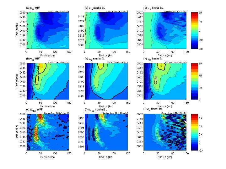
Boundary-layer evolution during ERC

How well does the BL model reproduce HNR 1? Low-pass filtered, azimuthal -mean WRF (left) Extract p at 2. 2 km height (top of BL model) Insert p in BL model and calculate equilibrium wind field (right) Structure very similar Diagnosed fields tend to underestimate strength of secondary circulation • No buoyancy!

w v 10 vgr -u 10 Diagnostic: solid WRF: dashed

Boundary-layer evolution during ERC The nonlinear, diagnostic analysis reproduces the time evolution of the boundary layer.

Sensitivity of the linear model to "wiggles"

Linear TCBL flow with V "wiggles" ζ V W 1 km v 10 -u 10 w’ ζ'

Nonlinear TCBL flow with V "wiggles" Nonlinear Linear ζ V w w’ ζ' v 10 -u 10

Spatial filtering • Inflowing air columns experience a change in the BL's parameters • Gradient wind, vorticity, surface roughness, etc • Columns adjust on time scale I, travel with velocity scale U, hence expect radial space scale U/I. • This effect is missing in the linearized BL model because radial advection of perturbation flow is removed. • Nonlinear BL model filters out the effects of small-scale (i. e. < U/I) perturbations in the gradient wind field

Normalised response amplitude Filter properties Nondimensional wavelength of perturbation • Relative response for various wavelength (lam) • i. e. amplitude in nonlinear model / amplitude in linear model • Short oscillations are almost eliminated • Longer ones retained (possible resonance in one case)
-2∂ζ/∂r Cd")
Where is the eyewall frictional updraft? • Linear analytic solution: updraft approximately -(ζ+f)-2∂ζ/∂r Cd V 2 • Peak updraft is located slightly outside of RMW • Nonlinear overshoot of inflow displaces the updraft inwards • But how far? • Physically and dimensionally, U/I is plausible displacement scale

Updraft location with secondary eyewalls • Distance between updraft and wind max is greater for outer eyewall than inner w • Does the U/I scaling apply? V v 10 -u 10

Eyewall updraft location, single eyewall • Location of eyewall updraft maximum at 500 -m height, relative to location of max vorticity gradient • 3 RMWs (15, 25, 40 km) • 4 intensities (20, 30, 50, 70 m s-1) • Vary Cd and K • Vary "peakedness" Increasing RMW

Eyewall updraft location, secondary eyewall • Inwards displacement of secondary eyewall updraft at 1 -km height (relative to ∂ζ/∂r extremum) • Various secondary RMWs (50 – 150 km) • Various strengths • Vary outer structure Increasing secondary RMW • Vary Cd and K

SEF/ERC in WRF “Nature Run”

Cause and effect in fluid dynamics • Diagnosing cause and effect is difficult because the equations are strongly coupled • E. g. advection terms, continuity equation • Rotating fluids are especially difficult • Coriolis and generalised Coriolis terms • So we use other methods to supplement momentum budget equations • Vorticity and PV equation • Sawyer-Eliassen equation • Diagnostic boundary layer models

If we claim that A causes B then removing A should remove B

Concentric eyewalls, nonlinear

Concentric eyewalls, linear

Removing the nonlinear terms … • Mostly removes the supergradient flow • Alters the strength and location of the inflow maxima • Alters the location and outwards slope of the updraft • But it doesn't eliminate the updraft • This result is inconsistent with the proposition that the supergradient flow causes the updraft

BL flow for modified Rankine vortex

Same vortex + small vorticity bump

Same vortex + larger vorticity bump

Adding/removing the vorticity bump … • Adds/removes the outer eyewall updraft • Creates/destroys outer inflow maximum • Strengthens/weakens supergradient flow near the bump • These effects increase for a stronger bump • Strong evidence that the vorticity perturbation causes these features

Conclusions Outer RMW is very efficient in producing frictional updrafts Because in environment of low vorticity Hypothesise SEF/ERC has boundary layer contribution through positive feedback Boundary-layer diagnostic model captures boundary-layer structure of WRF simulation Inwards displacement of eyewall frictional updraft scales as U/I, Greater displacement for larger RMW
- Slides: 52