Extratropical Sensitivity to Tropical SST Prashant Sardeshmukh Joe

Extratropical Sensitivity to Tropical SST Prashant Sardeshmukh, Joe Barsugli, and Sang-Ik Shin Climate Diagnostics Center

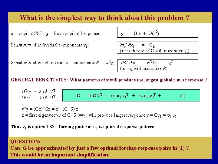
What is the simplest way to think about this problem ? x = tropical SST, y = Extratropical Response y = G x + O(x 2) Sensitivity of individual components yi : ∂yi/ ∂xj = Gij (x = i th row of G will maximize yi) Sensitivity of weighted sum of components R = w. Ty; ∂R/ ∂ xj = w. TG = g. T ( x = g will maximize R) Math slide 1 GENERAL SENSITIVITY: What patterns of x will produce the largest global r. m. s response ? G T G = V s 2 V T GGT = U s 2 UT G = U s VT = s 1 u 1 v 1 T + s 2 u 2 v 2 T +. . (1) y. Ty = (Gx)TGx = x. T (GTG) x x = first eigenvector of GTG (=v 1) will produce largest response y = Gv 1 = s 1 u 1 Thus v 1 is optimal SST forcing pattern; u 1 is optimal response pattern QUESTION: Can G be approximated by just a few optimal forcing-response pairs in (1) ? This would be an important simplification.

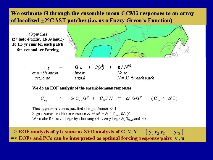
We estimate G through the ensemble-mean CCM 3 responses to an array of localized +2°C SST patches (i. e. as a Fuzzy Green’s Function) 43 patches (27 Indo-Pacific, 16 Atlantic) 16 1. 5 yr runs for each patch for +ve and -ve Forcing y = ensemble-mean response Gx + O(x 2) + linear signal e / N 1/2 Noise N = 32 for each patch We do an EOF analysis of the ensemble-mean responses. Cyy ≈ G Cxx GT + Cee / N ≈ a 2 GGT ( Cxx ≈ a 2 I ) Math slide 2 This approximation is justified if signal/noise >> 1 Signal variance / Noise variance N a 2 = N ( Tmax A )2 We make this ratio large by choosing relatively large N, Tmax and A => EOF analysis of y is same as SVD analysis of G ≈ Y = [ y 1 y 2 y 3. . . y 43 ] => EOFs and PCs can be interpreted as optimal forcing-response pairs v , u

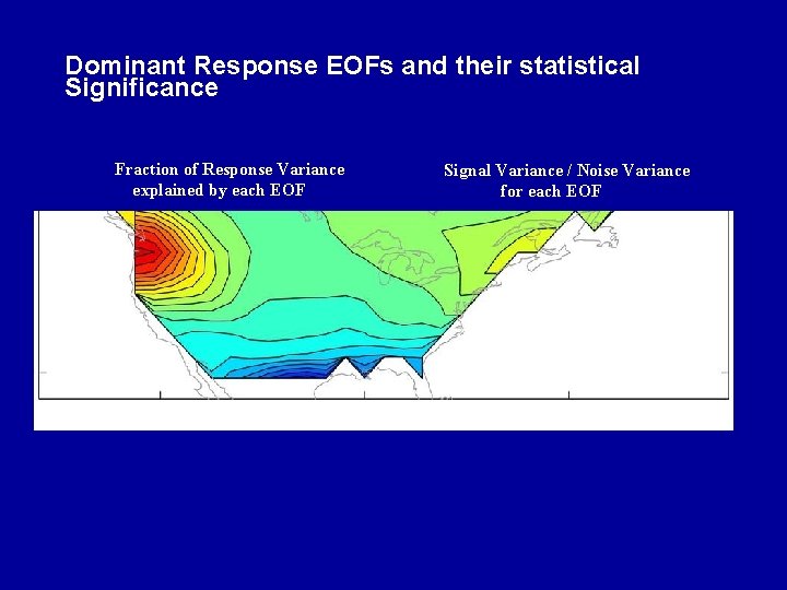
Dominant Response EOFs and their statistical Significance Fraction of Response Variance explained by each EOF Signal Variance / Noise Variance for each EOF

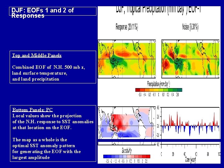
DJF: EOFs 1 and 2 of Responses Top and Middle Panels Combined EOF of N. H. 500 mb z, land surface temperature, and land precipitation Bottom Panels: PC Local values show the projection of the N. H. response to SST anomalies at that location on the EOF. The map as a whole is the optimal SST anomaly pattern for generating the EOF with the largest amplitude

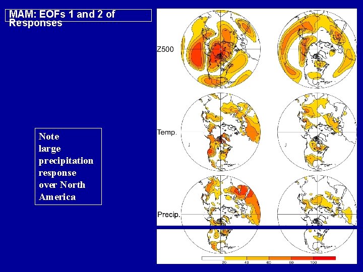
MAM: EOFs 1 and 2 of Responses Note large precipitation response over North America

JJA: EOFs 1 and 2 of Responses The 500 mb height response is weak in JJA, but there is still a large precipitation response

SON: EOFs 1 and 2 of Responses Both the 500 mb height and precipitation responses are weak in SON, although there is still an appreciable precipitation response over the central and southeast U. S.

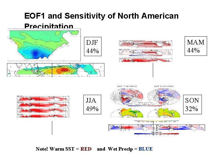
EOF 1 and Sensitivity of North American Precipitation DJF 44% MAM 44% JJA 49% SON 32% Note! Warm SST = RED and Wet Precip = BLUE

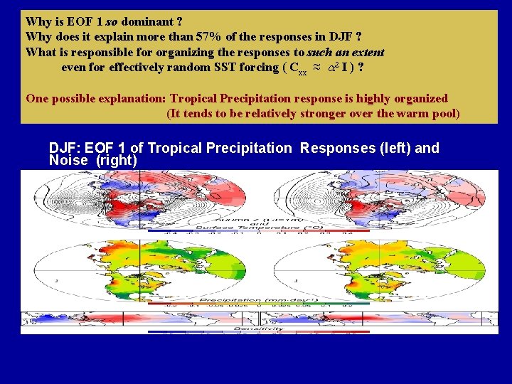
Why is EOF 1 so dominant ? Why does it explain more than 57% of the responses in DJF ? What is responsible for organizing the responses to such an extent even for effectively random SST forcing ( Cxx ≈ a 2 I ) ? One possible explanation: Tropical Precipitation response is highly organized (It tends to be relatively stronger over the warm pool) DJF: EOF 1 of Tropical Precipitation Responses (left) and Noise (right)

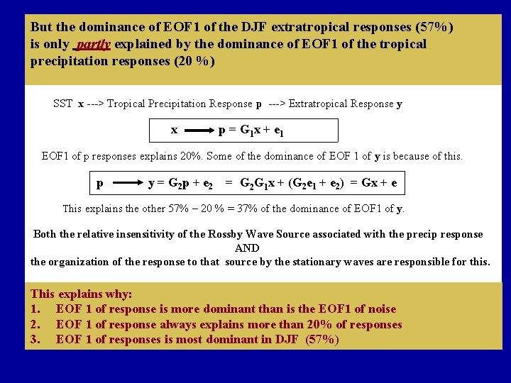
But the dominance of EOF 1 of the DJF extratropical responses (57%) is only partly explained by the dominance of EOF 1 of the tropical precipitation responses (20 %) SST x ---> Tropical Precipitation Response p ---> Extratropical Response y x p = G 1 x + e 1 EOF 1 of p responses explains 20%. Some of the dominance of EOF 1 of y is because of this. p y = G 2 p + e 2 = G 2 G 1 x + (G 2 e 1 + e 2) = Gx + e This explains the other 57% - 20 % = 37% of the dominance of EOF 1 of y. Both the relative insensitivity of the Rossby Wave Source associated with the precip response Math slide 3 AND the organization of the response to that source by the stationary waves are responsible for this. This explains why: 1. EOF 1 of response is more dominant than is the EOF 1 of noise 2. EOF 1 of response always explains more than 20% of responses 3. EOF 1 of responses is most dominant in DJF (57%)

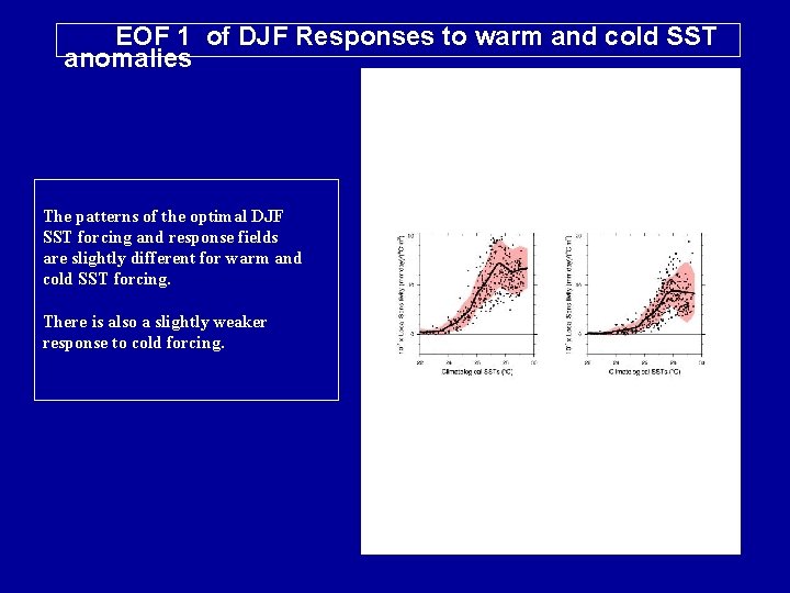
What about Nonlinearity ? How Important is it ? Sensitivity of Local Tropical Precipitation Response (as a function of background SST) For +2° C anomalies For - 2° C anomalies

EOF 1 of DJF Responses to warm and cold SST anomalies The patterns of the optimal DJF SST forcing and response fields are slightly different for warm and cold SST forcing. There is also a slightly weaker response to cold forcing.

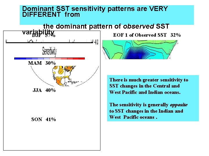
Dominant SST sensitivity patterns are VERY DIFFERENT from the dominant pattern of observed SST variability EOF 1 of Observed SST 32% DJF 57% MAM 30% JJA 40% There is much greater sensitivity to SST changes in the Central and West Pacific and Indian oceans. SON 41% The sensitivity is generally opposite to SST changes in the Indian and West Pacific oceans.

Summar y 1. 2. Extratropical sensitivity to tropical SST changes can be characterized by just 2 or 3 optimal forcing-response pairs in each season. 2. The dominance of these pairs results partly from the relatively large sensitivity of the local precipitation response in regions of warmer background SST such as the warm pool, and partly from a “modal” dynamical extratropical response to tropical diabatic forcing (Ting and Sardeshmukh 1993). 3. The optimal SST forcing patterns are VERY DIFFERENT from the ENSO pattern. The only area of significant overlap is Nino-4. The extratropical climate generally shows opposite sensitivities to SST changes in the western and eastern halves of the warm pool. 5. 6. 5. These results have important implications for understanding and modeling global climate changes from monthly to millenial time scales.

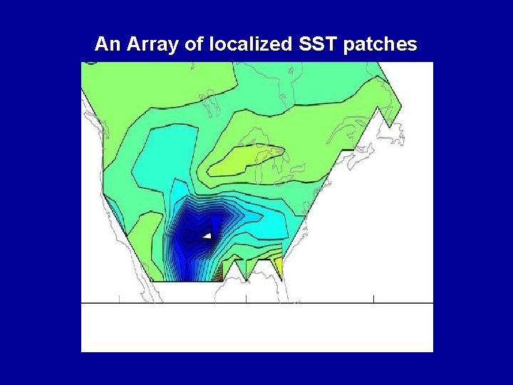
An Array of localized SST patches

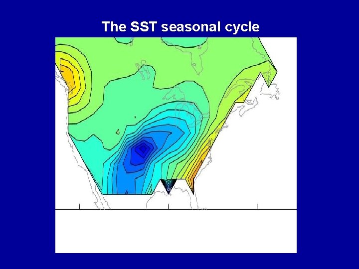
The SST seasonal cycle

DJF: Local Variance Explained by Response EOFs 1 and 2