Extracting templates for Natural Scene Classification Content Based

Extracting templates for Natural Scene Classification

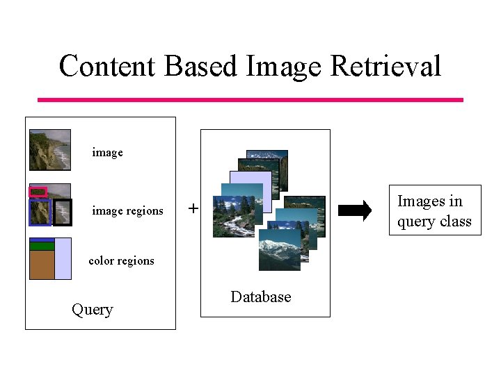
Content Based Image Retrieval image regions Images in query class + color regions Query Database

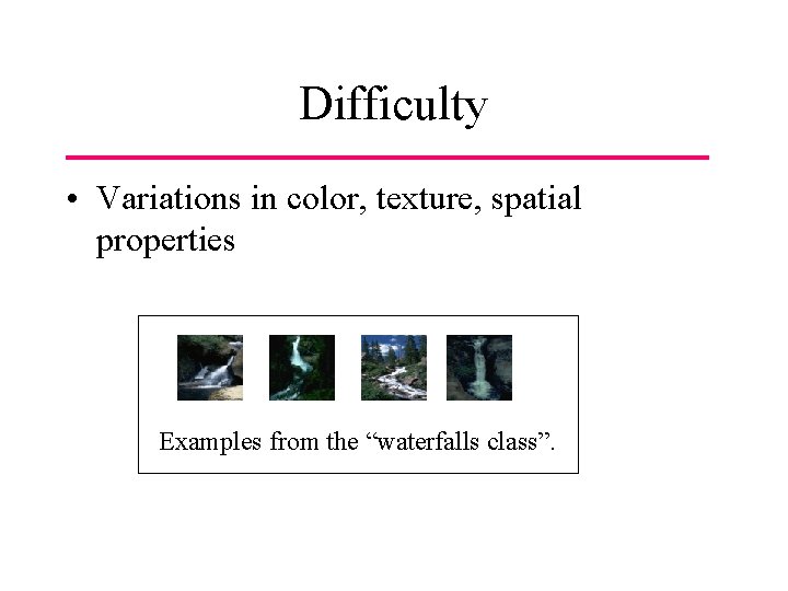
Difficulty • Variations in color, texture, spatial properties Examples from the “waterfalls class”.

Configural Recognition (Lipson 1996) • Predefined templates : – relative spatial and photometric properties between image regions – low resolution – global configuration of image regions

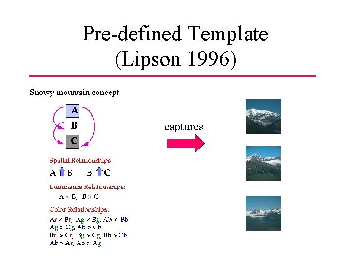
Pre-defined Template (Lipson 1996) Snowy mountain concept captures

Template Extraction [r 1, g 1, b 1] EXAMPLE IMAGE INSTANCES 1 4 Downsample and generate instances 2 3 [r 2, g 2, b 2] Instance=[x, y, r, g, b, r 1, g 1, b 1, r 2, g 2, b 2, …. r 4, g 4, b 4] r 1, g 1, b 1 are differences in mean color between central blob and blob above it. . . TEMPLATE EXTRACTION 1. Downsample example images 2. Extract all instances from each example image 3. Find the set of all instances that are common (reinforced) in all the positive examples (discrete intersection) 4. The common instances and their spatial relationship is the extracted template CLASSIFICATION For every instance in the template find closest match in new image that satisfy color and spatial relationships.

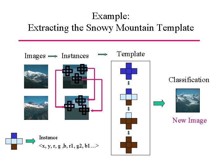
Example: Extracting the Snowy Mountain Template Images Instances Template Classification New Image Instance <x, y, r, g , b, r 1, g 2, b 1…>

Multiple-Instance learning for Natural Scene Classification Oded Maron and Aparna Lakshmi Ratan

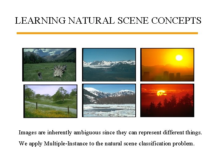
LEARNING NATURAL SCENE CONCEPTS Images are inherently ambiguous since they can represent different things. We apply Multiple-Instance to the natural scene classification problem.

Multiple Instance Learning • Regular learning: learn concept form leabeled examples • MI learning: learn concepts from labeled bags • a bag is a collection of examples • positive bag has at least one positive example • negative bag has only negative examples

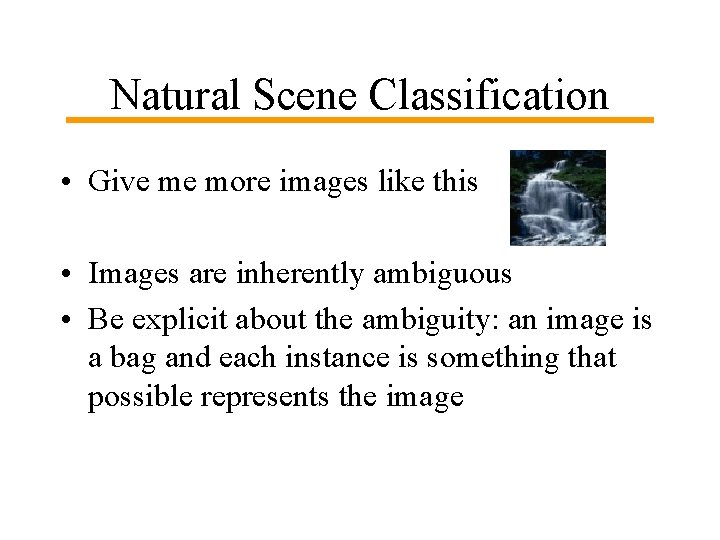
Natural Scene Classification • Give me more images like this • Images are inherently ambiguous • Be explicit about the ambiguity: an image is a bag and each instance is something that possible represents the image

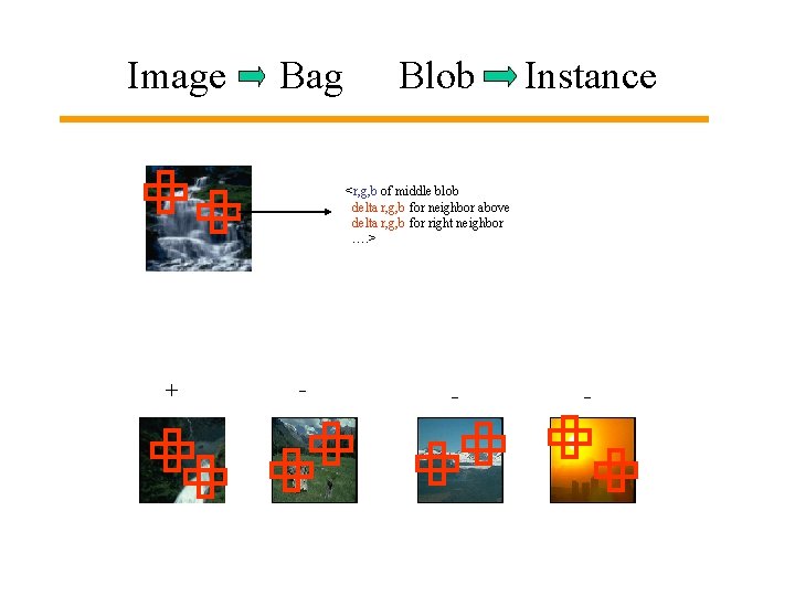
Image Bag Blob Instance <r, g, b of middle blob delta r, g, b for neighbor above delta r, g, b for right neighbor …. > + - - -

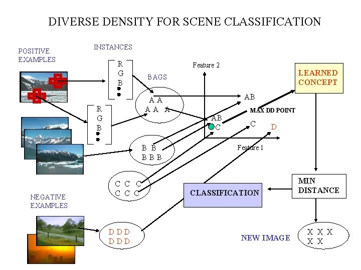
DIVERSE DENSITY FOR SCENE CLASSIFICATION POSITIVE EXAMPLES INSTANCES R G B Feature 2 AA AA A R G B BBB NEGATIVE EXAMPLES C C C DDD LEARNED CONCEPT BAGS AB AB C MAX DD POINT C D Feature 1 CLASSIFICATION NEW IMAGE MIN DISTANCE X X X

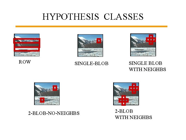
HYPOTHESIS CLASSES ROW SINGLE-BLOB 2 -BLOB-NO-NEIGHBS SINGLE BLOB WITH NEIGHBS 2 -BLOB WITH NEIGHBS

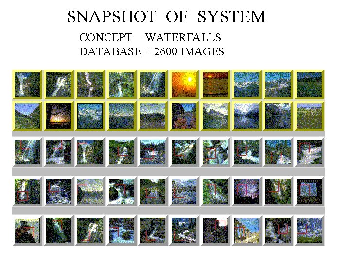
SNAPSHOT OF SYSTEM CONCEPT = WATERFALLS DATABASE = 2600 IMAGES

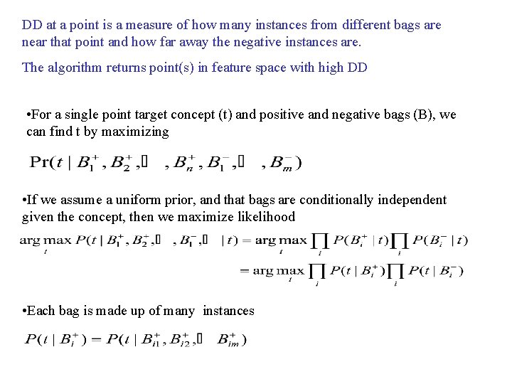
DD at a point is a measure of how many instances from different bags are near that point and how far away the negative instances are. The algorithm returns point(s) in feature space with high DD • For a single point target concept (t) and positive and negative bags (B), we can find t by maximizing • If we assume a uniform prior, and that bags are conditionally independent given the concept, then we maximize likelihood • Each bag is made up of many instances

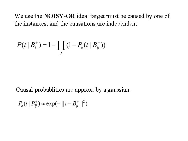
We use the NOISY-OR idea: target must be caused by one of the instances, and the causations are independent Causal probablities are approx. by a gaussian.

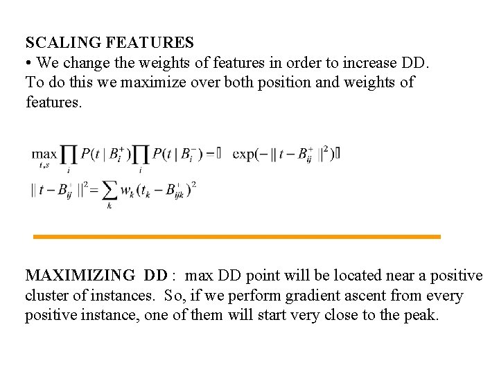
SCALING FEATURES • We change the weights of features in order to increase DD. To do this we maximize over both position and weights of features. MAXIMIZING DD : max DD point will be located near a positive cluster of instances. So, if we perform gradient ascent from every positive instance, one of them will start very close to the peak.

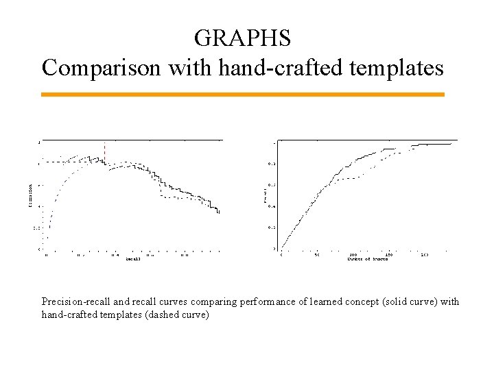
GRAPHS Comparison with hand-crafted templates Precision-recall and recall curves comparing performance of learned concept (solid curve) with hand-crafted templates (dashed curve)

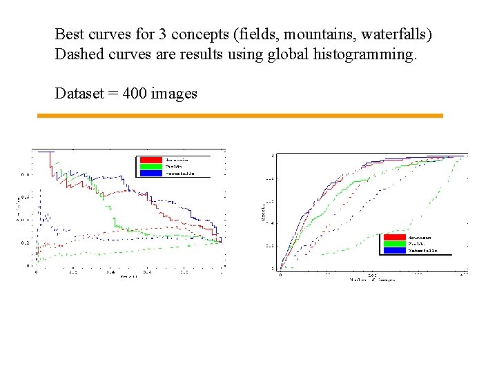
Best curves for 3 concepts (fields, mountains, waterfalls) Dashed curves are results using global histogramming. Dataset = 400 images

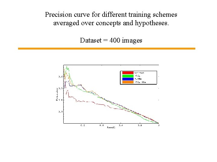
Precision curve for different training schemes averaged over concepts and hypotheses. Dataset = 400 images

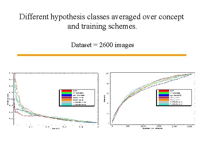
Different hypothesis classes averaged over concept and training schemes. Dataset = 2600 images

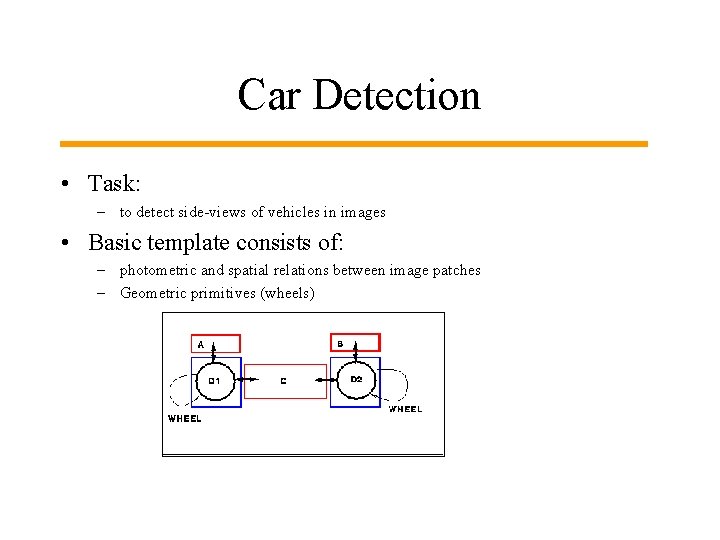
Car Detection • Task: – to detect side-views of vehicles in images • Basic template consists of: – photometric and spatial relations between image patches – Geometric primitives (wheels)

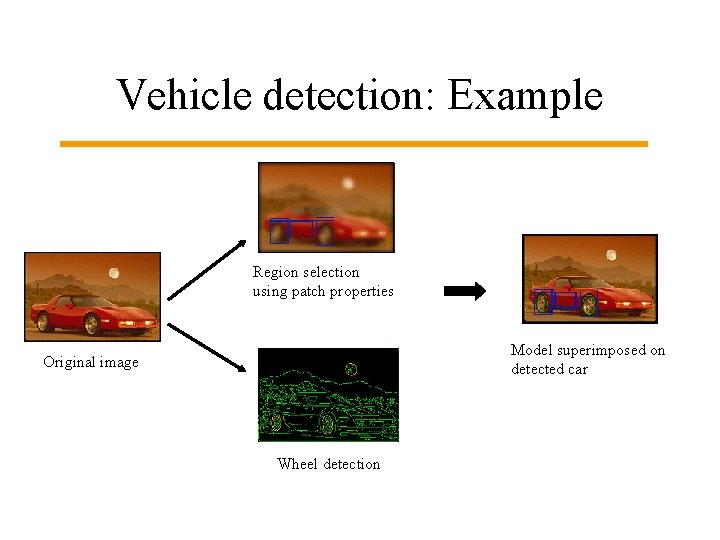
Vehicle detection: Example Region selection using patch properties Model superimposed on detected car Original image Wheel detection

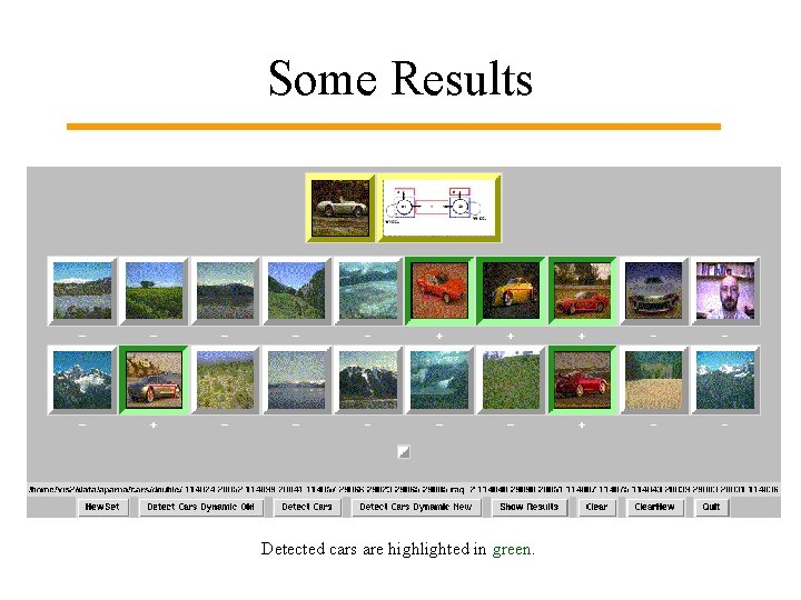
Some Results Detected cars are highlighted in green.

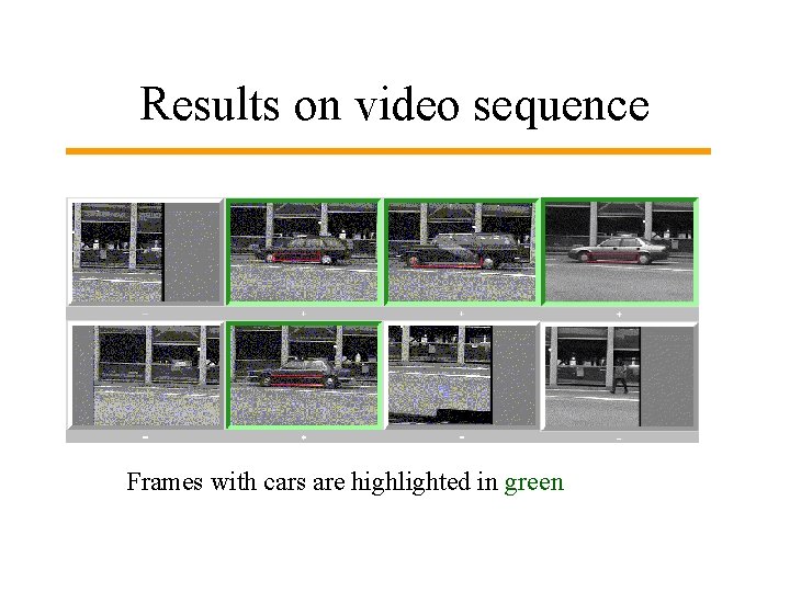
Results on video sequence Frames with cars are highlighted in green