Extra material for DAA 18 2 2016 How

Extra material for DAA++ 18. 2. 2016 How to cluster data Algorithm review Prof. Pasi Fränti Speech & Image Processing Unit School of Computing University of Eastern Finland Joensuu, FINLAND

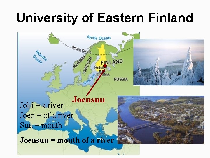
University of Eastern Finland Joensuu Joki = a river Joen = of a river Suu = mouth Joensuu = mouth of a river

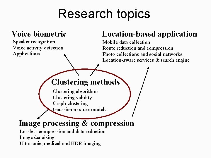
Research topics Voice biometric Location-based application Speaker recognition Voice activity detection Applications Mobile data collection Route reduction and compression Photo collections and social networks Location-aware services & search engine Clustering methods Clustering algorithms Clustering validity Graph clustering Gaussian mixture models Image processing & compression Lossless compression and data reduction Image denoising Ultrasonic, medical and HDR imaging

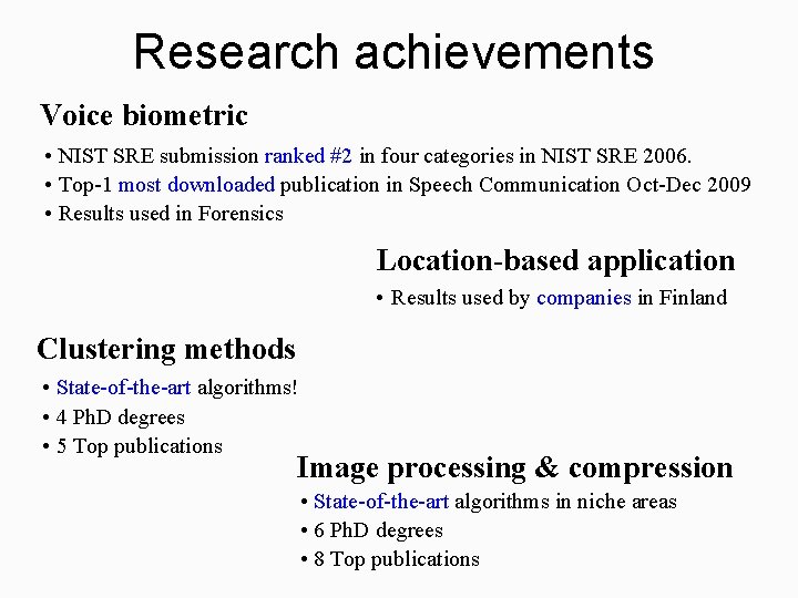
Research achievements Voice biometric • NIST SRE submission ranked #2 in four categories in NIST SRE 2006. • Top-1 most downloaded publication in Speech Communication Oct-Dec 2009 • Results used in Forensics Location-based application • Results used by companies in Finland Clustering methods • State-of-the-art algorithms! • 4 Ph. D degrees • 5 Top publications Image processing & compression • State-of-the-art algorithms in niche areas • 6 Ph. D degrees • 8 Top publications

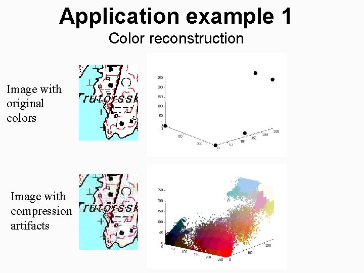
Application example 1 Color reconstruction Image with original colors Image with compression artifacts

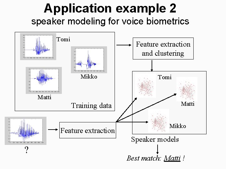
Application example 2 speaker modeling for voice biometrics Tomi Feature extraction and clustering Mikko Tomi Matti Training data Feature extraction Mikko Speaker models ? Best match: Matti !

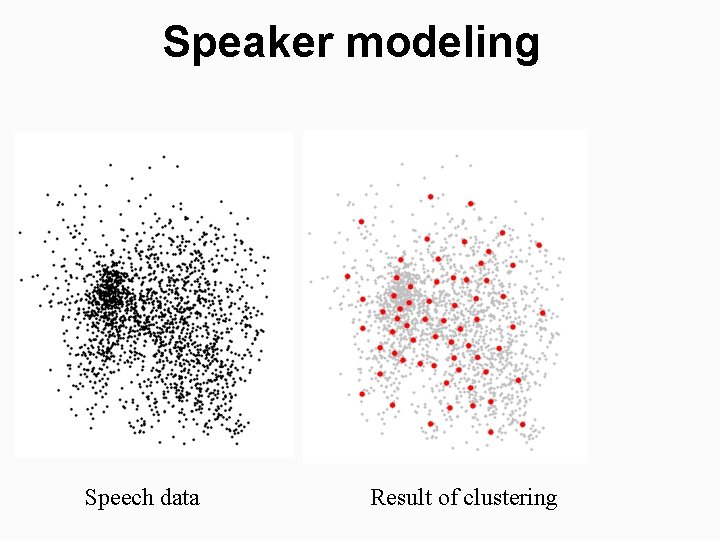
Speaker modeling Speech data Result of clustering

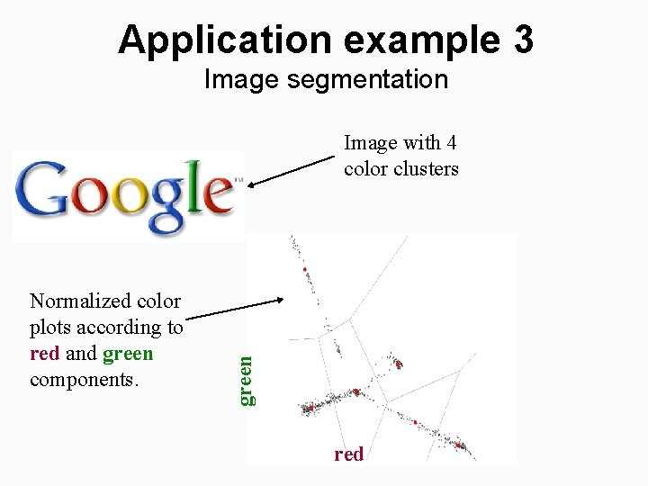
Application example 3 Image segmentation Normalized color plots according to red and green components. green Image with 4 color clusters red

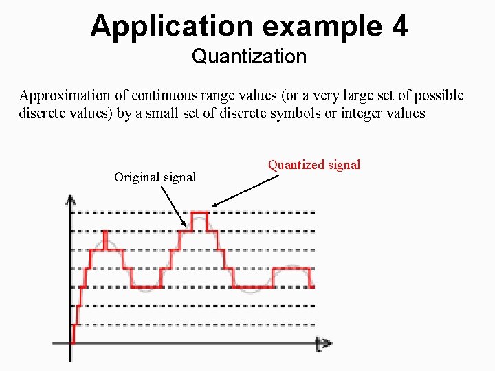
Application example 4 Quantization Approximation of continuous range values (or a very large set of possible discrete values) by a small set of discrete symbols or integer values Original signal Quantized signal

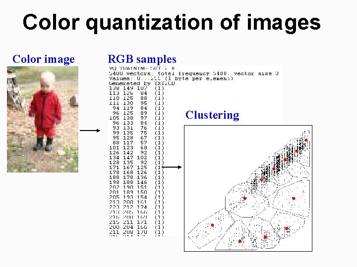
Color quantization of images Color image RGB samples Clustering

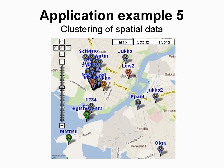
Application example 5 Clustering of spatial data

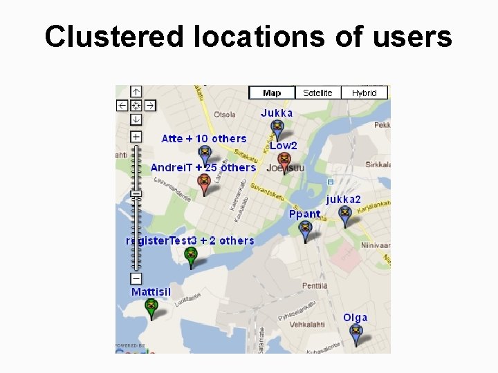
Clustered locations of users

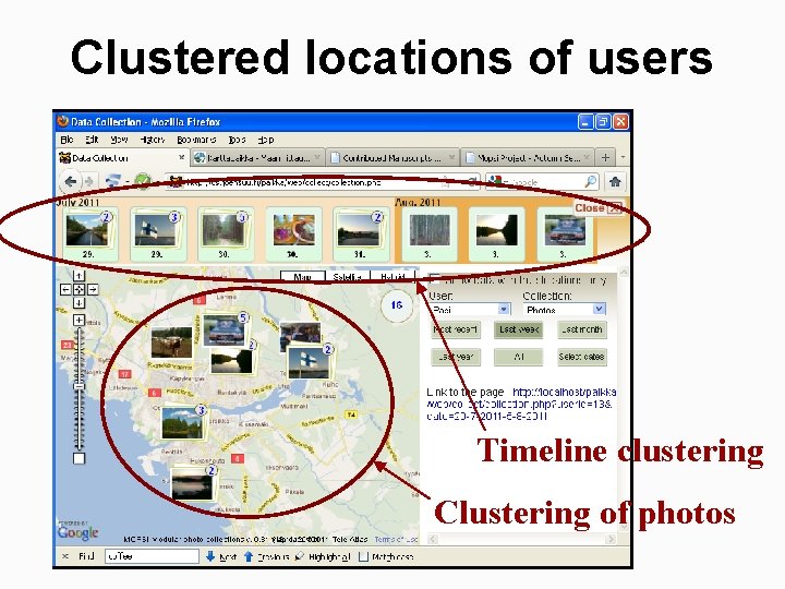
Clustered locations of users Timeline clustering Clustering of photos

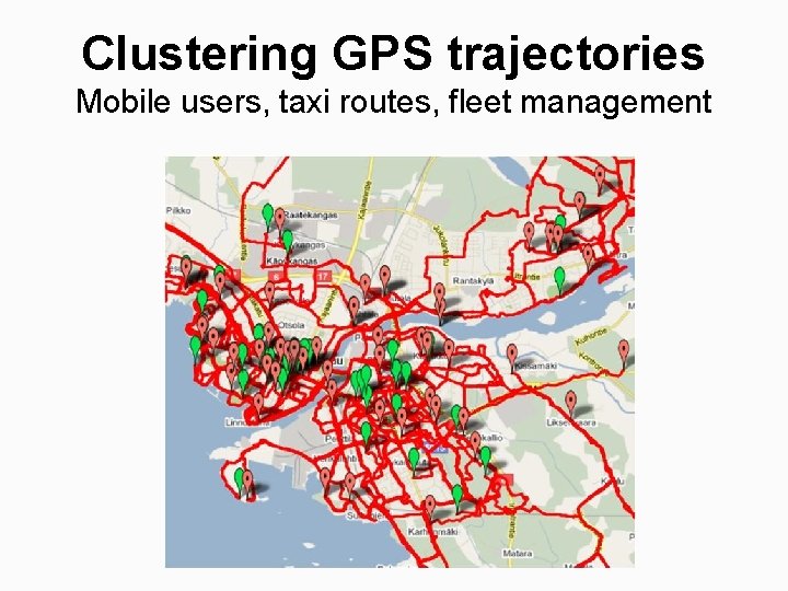
Clustering GPS trajectories Mobile users, taxi routes, fleet management

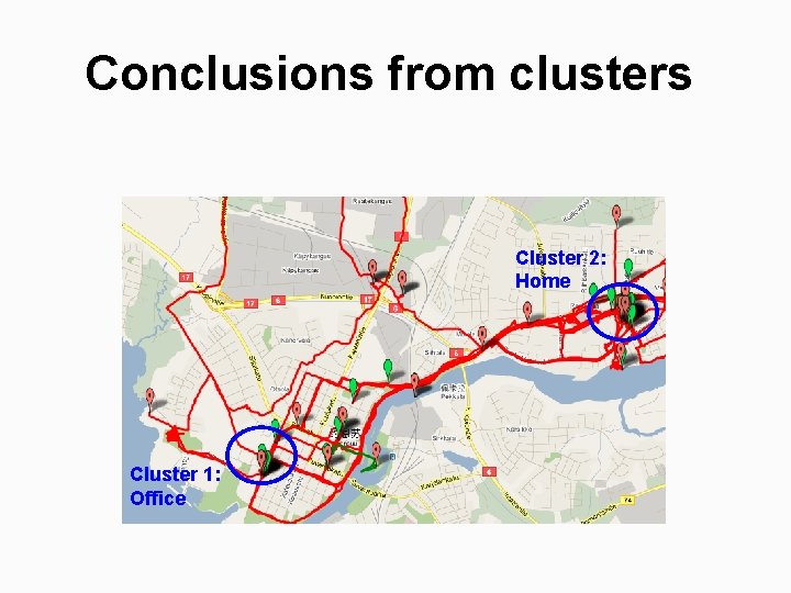
Conclusions from clusters Cluster 2: Home Cluster 1: Office

Part I: Clustering problem

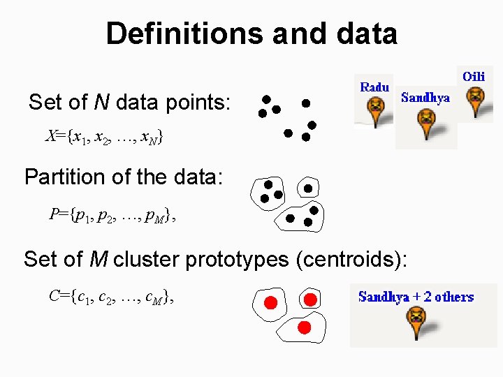
Definitions and data Set of N data points: X={x 1, x 2, …, x. N} Partition of the data: P={p 1, p 2, …, p. M}, Set of M cluster prototypes (centroids): C={c 1, c 2, …, c. M},

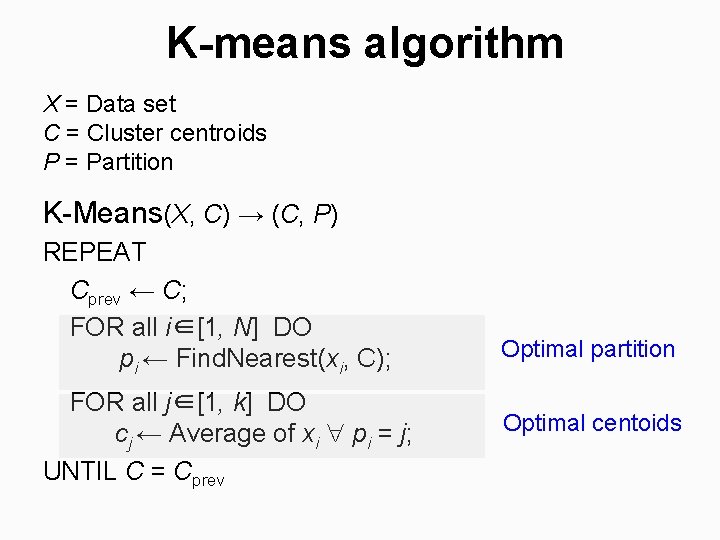
K-means algorithm X = Data set C = Cluster centroids P = Partition K-Means(X, C) → (C, P) REPEAT Cprev ← C; FOR all i∈[1, N] DO pi ← Find. Nearest(xi, C); FOR all j∈[1, k] DO cj ← Average of xi pi = j; UNTIL C = Cprev Optimal partition Optimal centoids

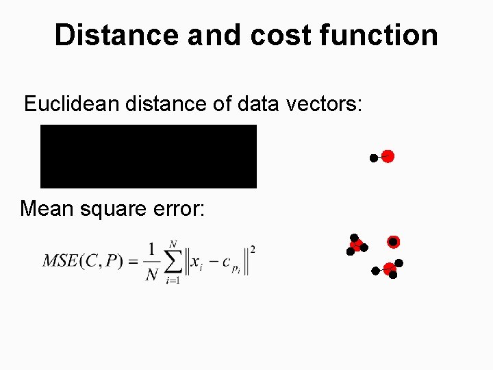
Distance and cost function Euclidean distance of data vectors: Mean square error:

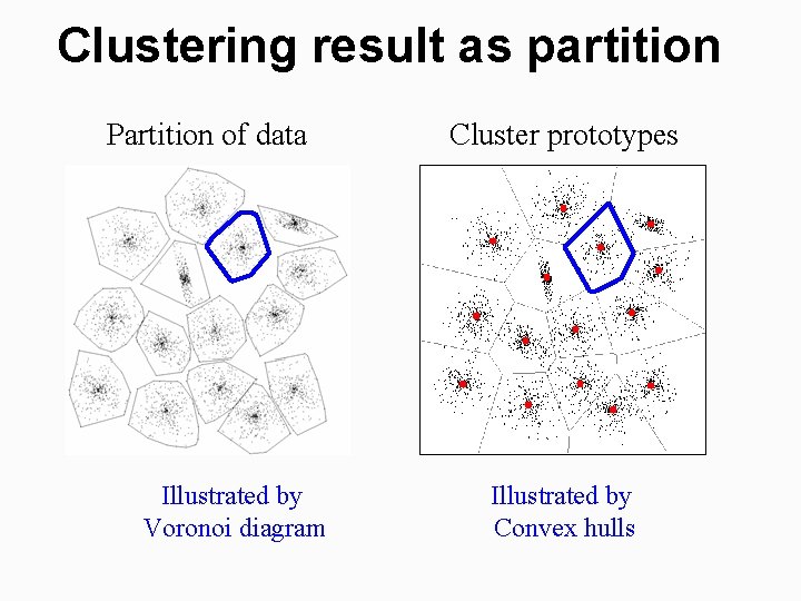
Clustering result as partition Partition of data Illustrated by Voronoi diagram Cluster prototypes Illustrated by Convex hulls

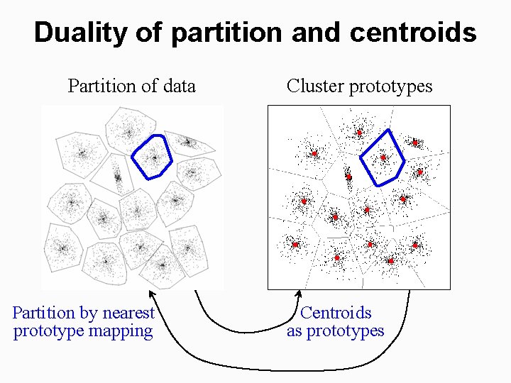
Duality of partition and centroids Partition of data Partition by nearest prototype mapping Cluster prototypes Centroids as prototypes

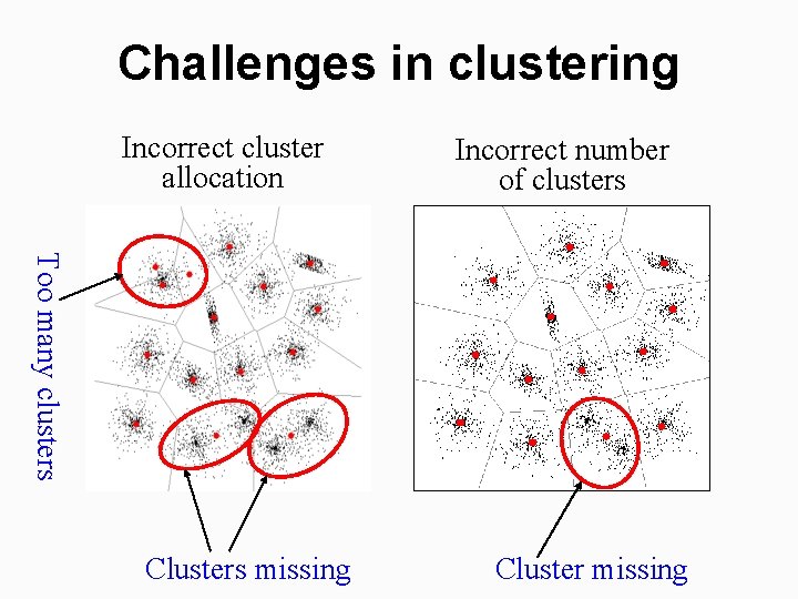
Challenges in clustering Incorrect cluster allocation Incorrect number of clusters Too many clusters Clusters missing Cluster missing

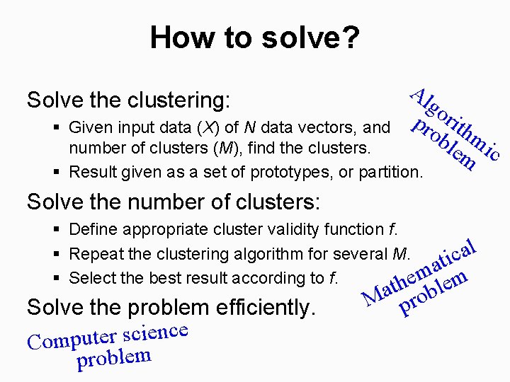
How to solve? Solve the clustering: Al go pr rith ob m lem ic § Given input data (X) of N data vectors, and number of clusters (M), find the clusters. § Result given as a set of prototypes, or partition. Solve the number of clusters: § Define appropriate cluster validity function f. l a § Repeat the clustering algorithm for several M. c i t a m § Select the best result according to f. he em Solve the problem efficiently. e c n e i c s r e t u Comp problem t obl a M pr

Part II: Clustering algorithms

Algorithm 1: Split P. Fränti, T. Kaukoranta and O. Nevalainen, "On the splitting method for vector quantization codebook generation", Optical Engineering, 36 (11), 3043 -3051, November 1997.

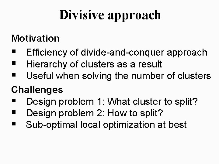
Divisive approach Motivation § Efficiency of divide-and-conquer approach § Hierarchy of clusters as a result § Useful when solving the number of clusters Challenges § Design problem 1: What cluster to split? § Design problem 2: How to split? § Sub-optimal local optimization at best

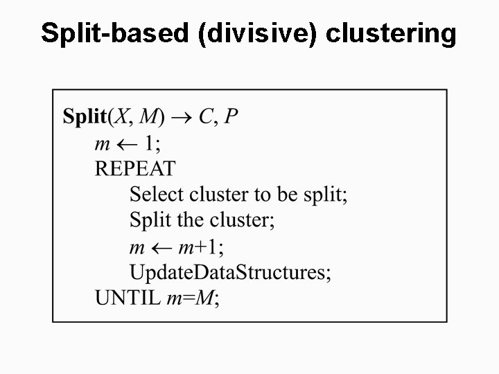
Split-based (divisive) clustering

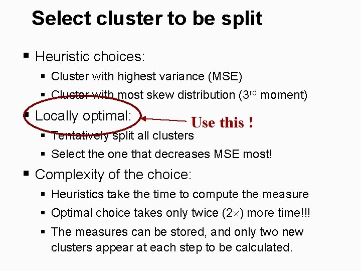
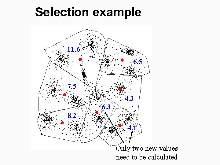
Select cluster to be split § Heuristic choices: § Cluster with highest variance (MSE) § Cluster with most skew distribution (3 rd moment) § Locally optimal: Use this ! § Tentatively split all clusters § Select the one that decreases MSE most! § Complexity of the choice: § Heuristics take the time to compute the measure § Optimal choice takes only twice (2 ) more time!!! § The measures can be stored, and only two new clusters appear at each step to be calculated.

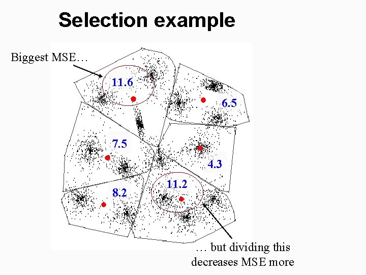
Selection example Biggest MSE… 11. 6 6. 5 7. 5 4. 3 8. 2 11. 2 … but dividing this decreases MSE more

Selection example 11. 6 6. 5 7. 5 4. 3 6. 3 8. 2 4. 1 Only two new values need to be calculated

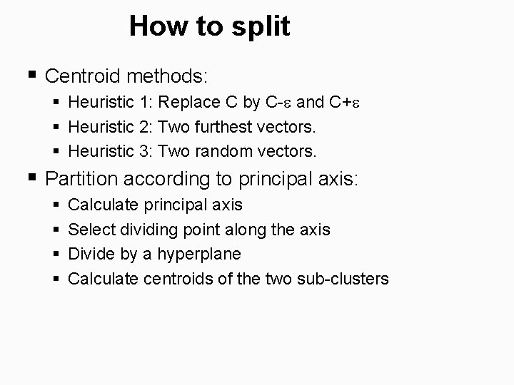
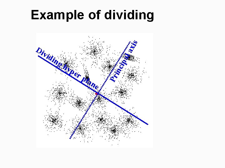
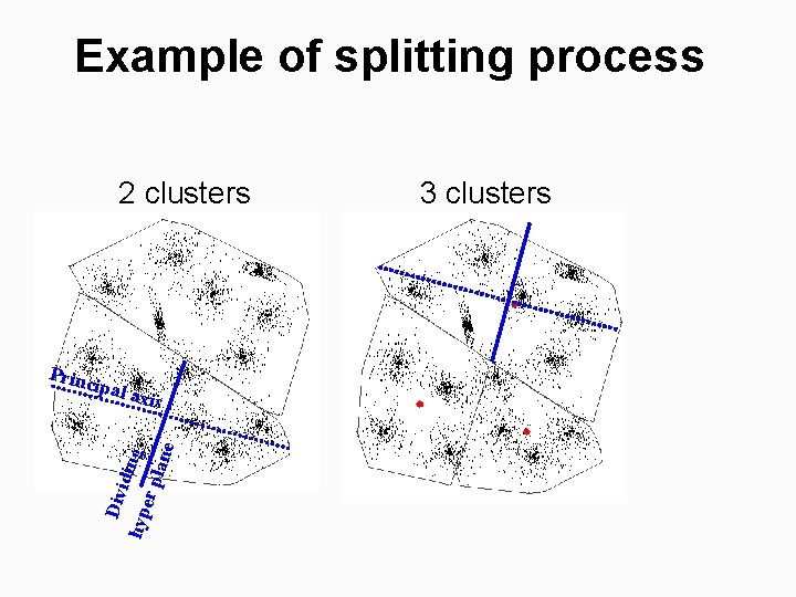
How to split § Centroid methods: § Heuristic 1: Replace C by C- and C+ § Heuristic 2: Two furthest vectors. § Heuristic 3: Two random vectors. § Partition according to principal axis: § § Calculate principal axis Select dividing point along the axis Divide by a hyperplane Calculate centroids of the two sub-clusters

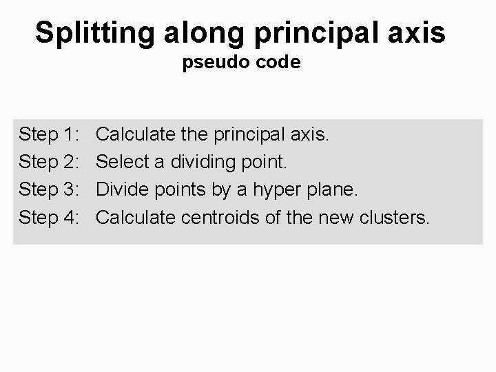
Splitting along principal axis pseudo code Step 1: Step 2: Step 3: Step 4: Calculate the principal axis. Select a dividing point. Divide points by a hyper plane. Calculate centroids of the new clusters.

pe r ipa hy pla inc ing la vid ne Pr Di xis Example of dividing

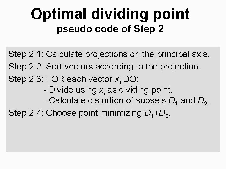
Optimal dividing point pseudo code of Step 2. 1: Calculate projections on the principal axis. Step 2. 2: Sort vectors according to the projection. Step 2. 3: FOR each vector xi DO: - Divide using xi as dividing point. - Calculate distortion of subsets D 1 and D 2. Step 2. 4: Choose point minimizing D 1+D 2.

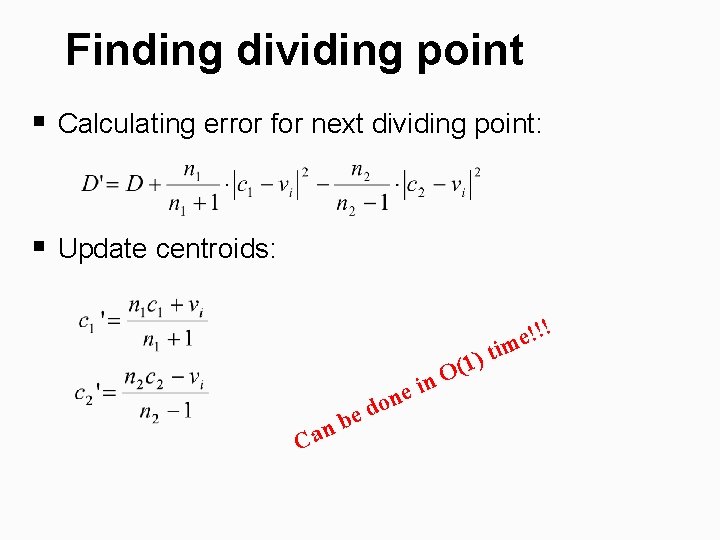
Finding dividing point § Calculating error for next dividing point: § Update centroids: e C b an in e don ) 1 ( O t !!! e im

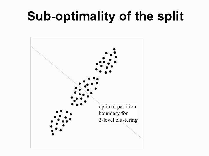
Sub-optimality of the split

Example of splitting process 2 clusters Princ ipal a Div idin g hyp er p lane xis 3 clusters

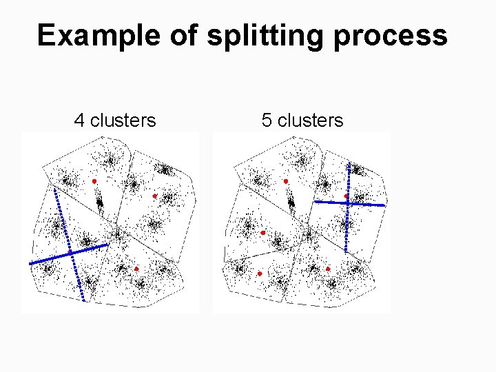
Example of splitting process 4 clusters 5 clusters

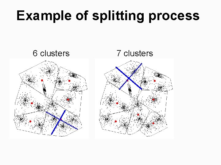
Example of splitting process 6 clusters 7 clusters

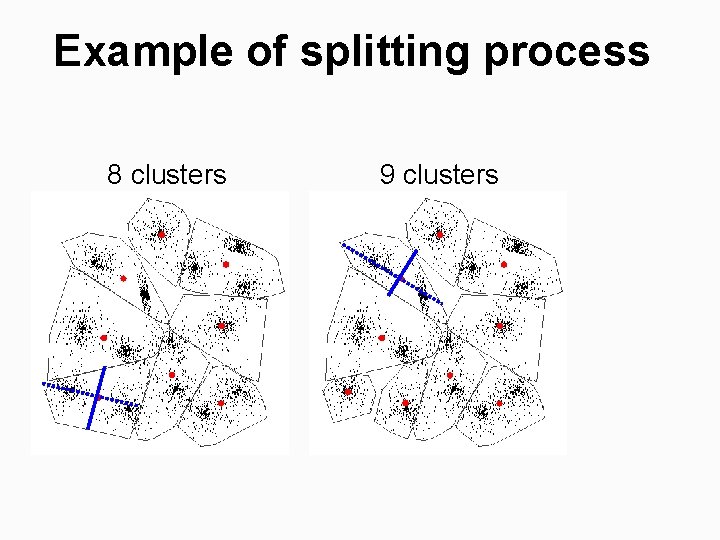
Example of splitting process 8 clusters 9 clusters

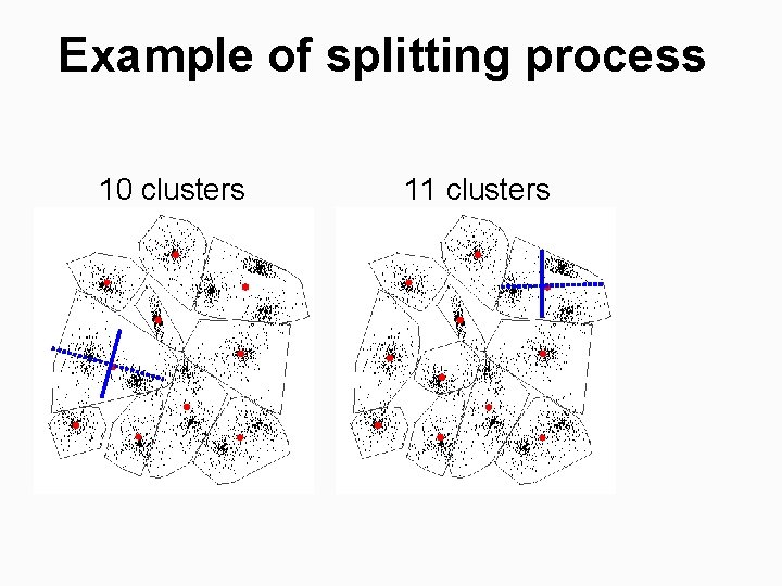
Example of splitting process 10 clusters 11 clusters

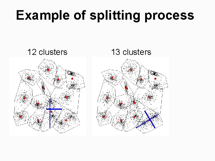
Example of splitting process 12 clusters 13 clusters

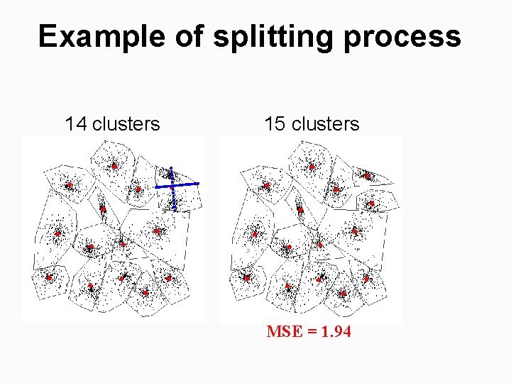
Example of splitting process 14 clusters 15 clusters MSE = 1. 94

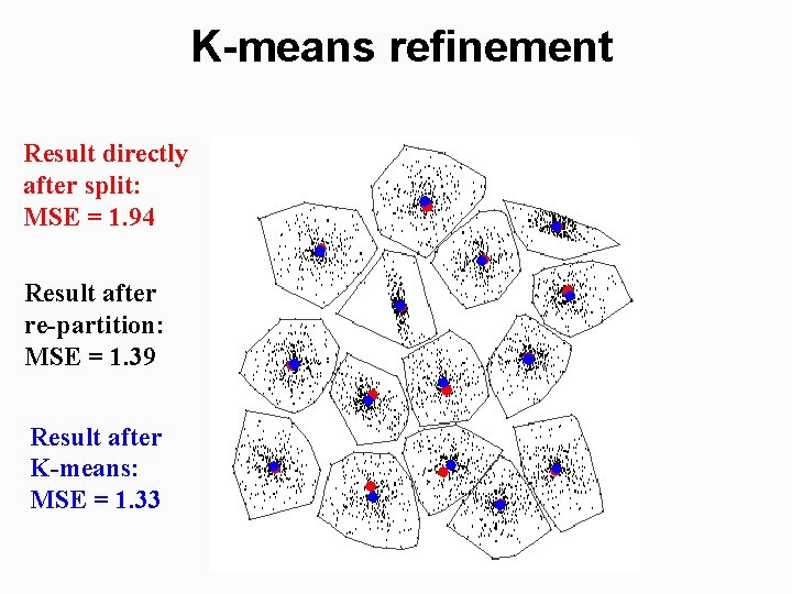
K-means refinement Result directly after split: MSE = 1. 94 Result after re-partition: MSE = 1. 39 Result after K-means: MSE = 1. 33

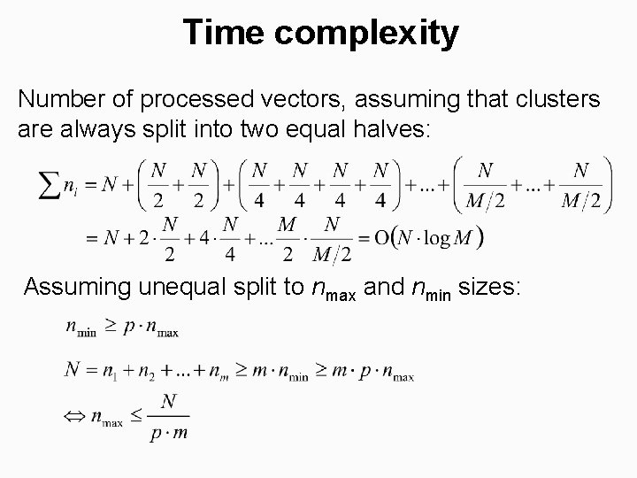
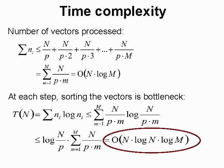
Time complexity Number of processed vectors, assuming that clusters are always split into two equal halves: Assuming unequal split to nmax and nmin sizes:

Time complexity Number of vectors processed: At each step, sorting the vectors is bottleneck:

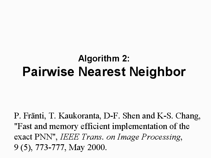
Algorithm 2: Pairwise Nearest Neighbor P. Fränti, T. Kaukoranta, D-F. Shen and K-S. Chang, "Fast and memory efficient implementation of the exact PNN", IEEE Trans. on Image Processing, 9 (5), 773 -777, May 2000.

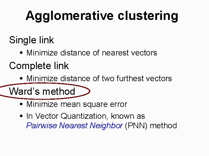
Agglomerative clustering Single link § Minimize distance of nearest vectors Complete link § Minimize distance of two furthest vectors Ward’s method § Minimize mean square error § In Vector Quantization, known as Pairwise Nearest Neighbor (PNN) method

PNN algorithm [Ward 1963: Journal of American Statistical Association] Merge cost: Local optimization strategy: Nearest neighbor search is needed: (1) finding the cluster pair to be merged (2) updating of NN pointers

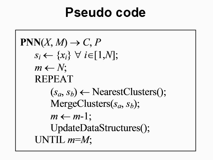
Pseudo code

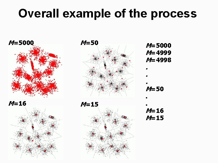
Overall example of the process M=5000 M=16 M=50 M=15 M=5000 M=4999 M=4998. . . M=50. . M=16 M=15

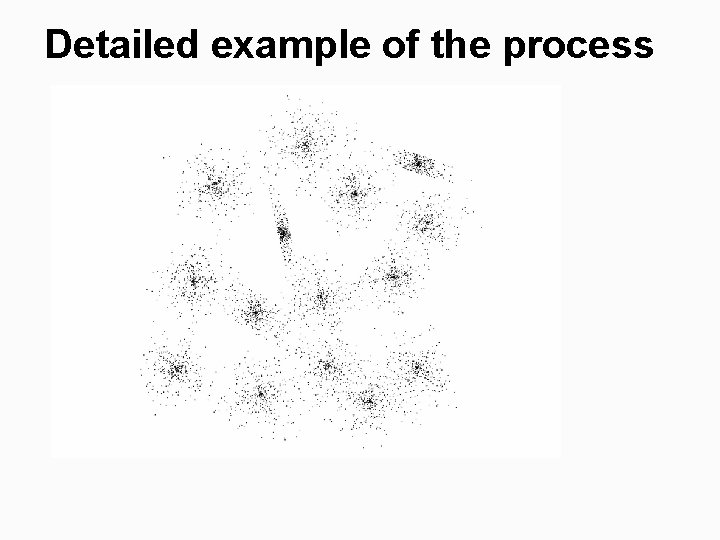
Detailed example of the process

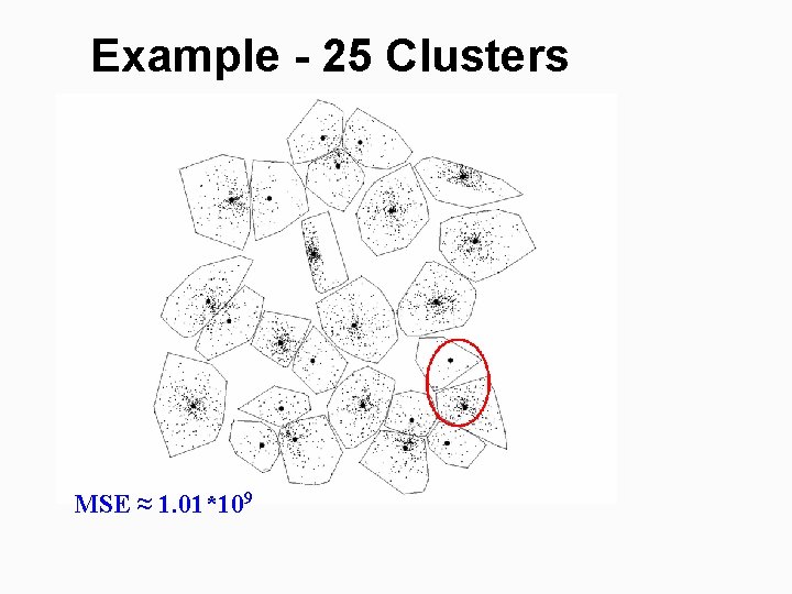
Example - 25 Clusters MSE ≈ 1. 01*109

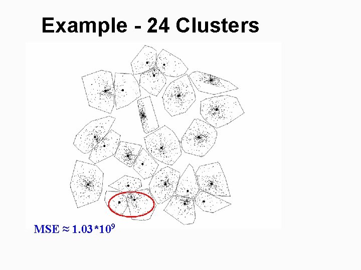
Example - 24 Clusters MSE ≈ 1. 03*109

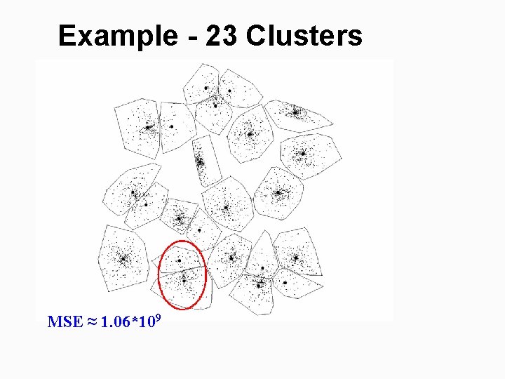
Example - 23 Clusters MSE ≈ 1. 06*109

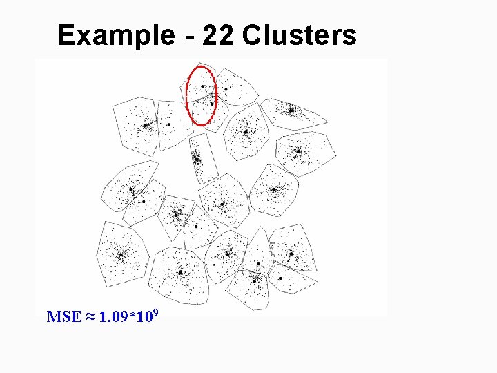
Example - 22 Clusters MSE ≈ 1. 09*109

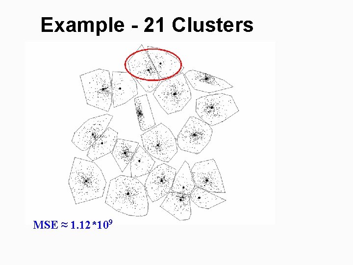
Example - 21 Clusters MSE ≈ 1. 12*109

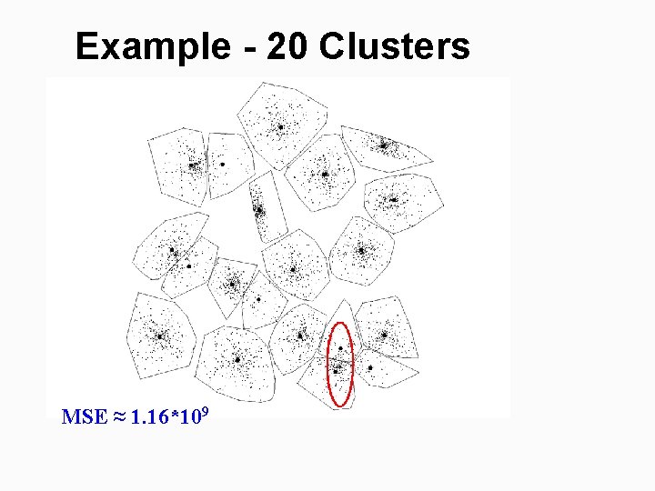
Example - 20 Clusters MSE ≈ 1. 16*109

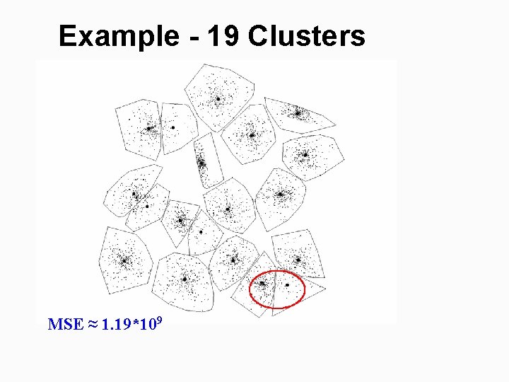
Example - 19 Clusters MSE ≈ 1. 19*109

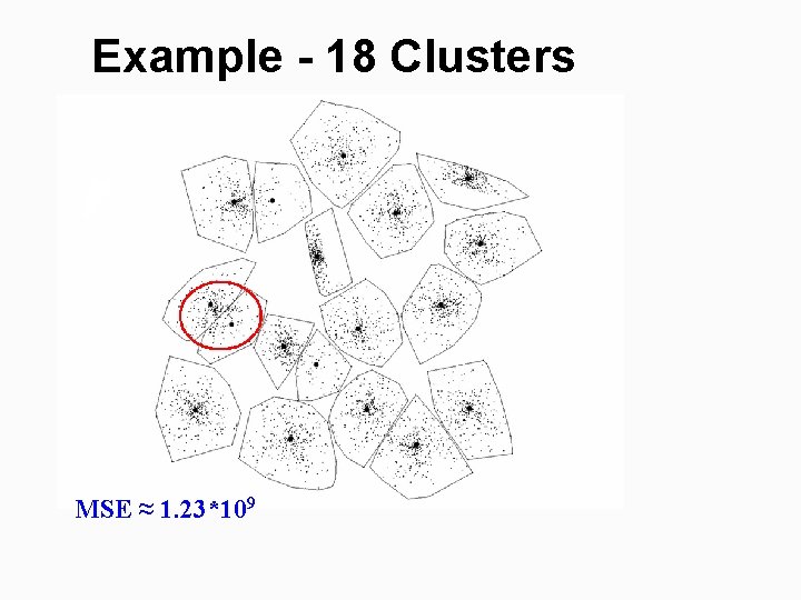
Example - 18 Clusters MSE ≈ 1. 23*109

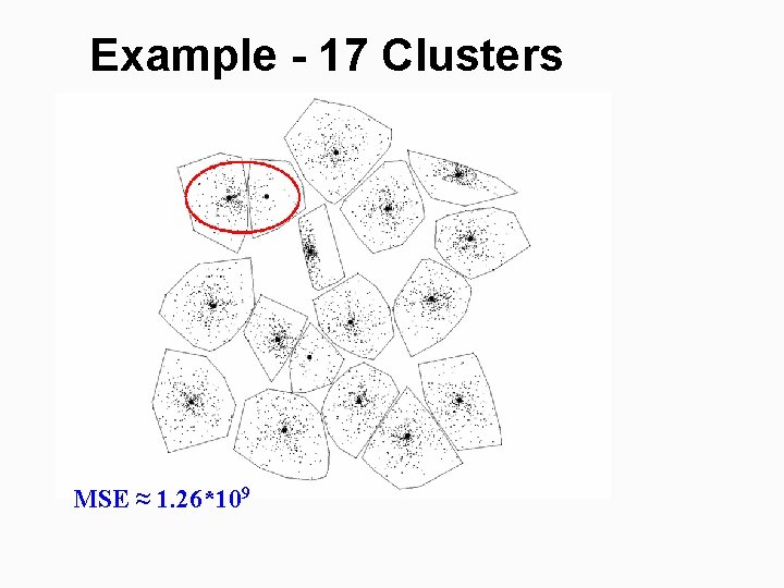
Example - 17 Clusters MSE ≈ 1. 26*109

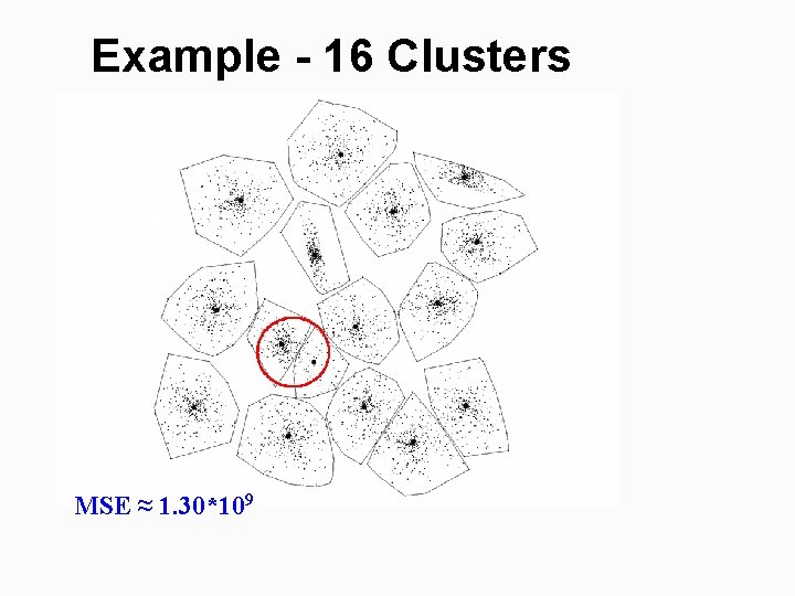
Example - 16 Clusters MSE ≈ 1. 30*109

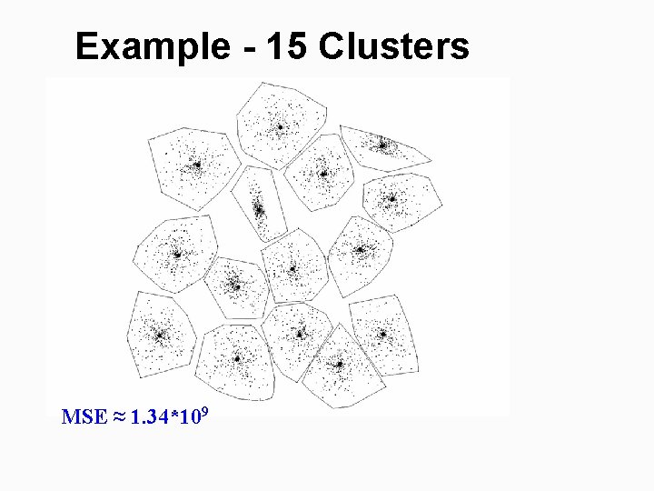
Example - 15 Clusters MSE ≈ 1. 34*109

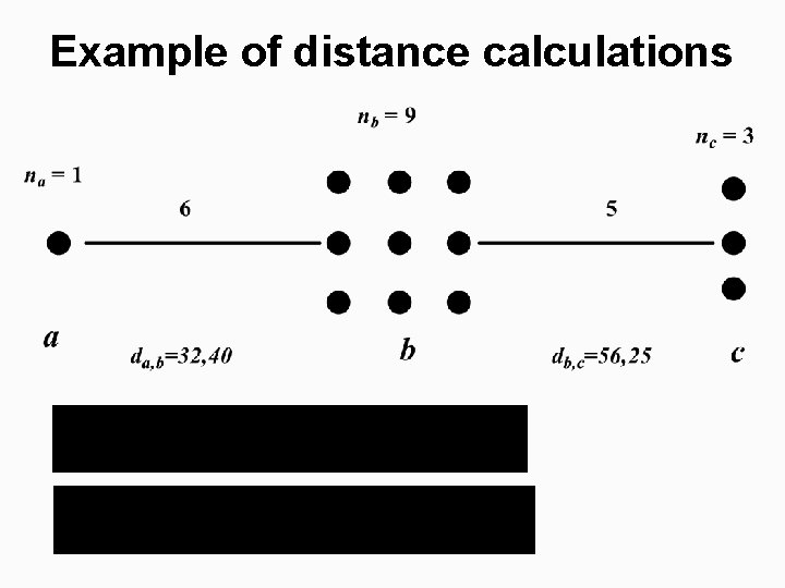
Example of distance calculations

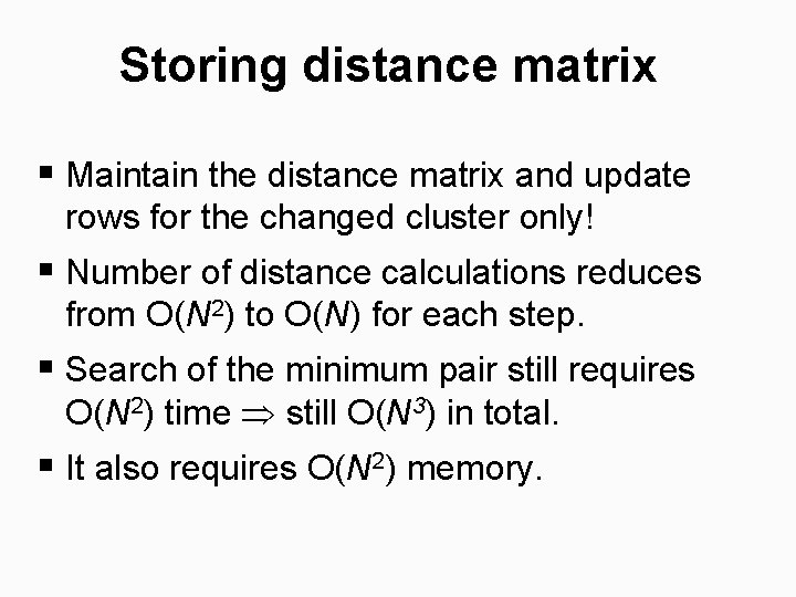
Storing distance matrix § Maintain the distance matrix and update rows for the changed cluster only! § Number of distance calculations reduces from O(N 2) to O(N) for each step. § Search of the minimum pair still requires O(N 2) time still O(N 3) in total. § It also requires O(N 2) memory.

Heap structure for fast search [Kurita 1991: Pattern Recognition] § Search reduces O(N) O(log. N). § In total: O(N 2 log. N)

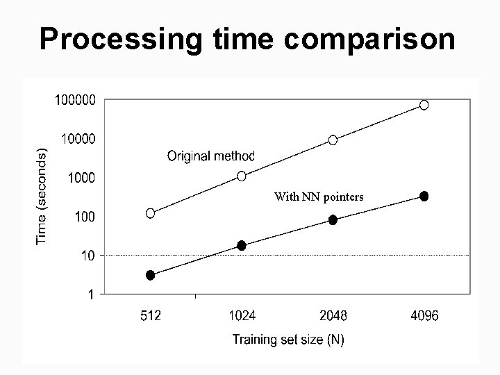
Maintain nearest neighbor (NN) pointers [Fränti et al. , 2000: IEEE Trans. Image Processing] Time complexity reduces to O(N 3) Ω ( N 2)

Processing time comparison With NN pointers

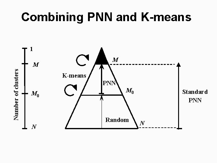
Combining PNN and K-means 1 M Number of clusters M K-means PNN M 0 Random N Standard PNN N

Further improvements § § P. Fränti, O. Virmajoki and V. Hautamäki, "Fast agglomerative clustering using a k-nearest neighbor graph". IEEE Trans. on Pattern Analysis and Machine Intelligence, 28 (11), 1875 -1881, November 2006. P. Fränti and O. Virmajoki, "Iterative shrinking method for clustering problems", Pattern Recognition, 39 (5), 761 -765, May 2006. T. Kaukoranta, P. Fränti and O. Nevalainen, "Vector quantization by lazy pairwise nearest neighbor method", Optical Engineering, 38 (11), 1862 -1868, November 1999. O. Virmajoki, P. Fränti and T. Kaukoranta, "Practical methods for speeding-up the pairwise nearest neighbor method ", Optical Engineering, 40 (11), 2495 -2504, November 2001.

Algorithm 3: Random Swap P. Fränti and J. Kivijärvi, "Randomised local search algorithm for the clustering problem", Pattern Analysis and Applications, 3 (4), 358 -369, 2000.

Random swap algorithm (RS)

Demonstration of the algorithm

Centroid swap

Local repartition

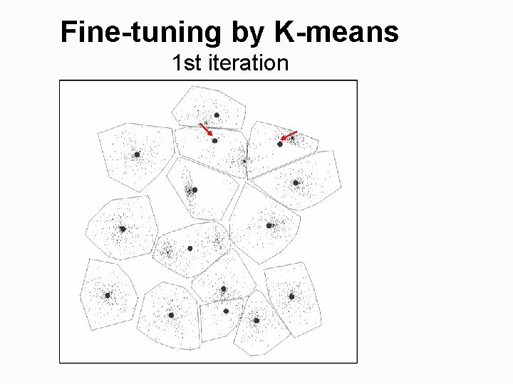
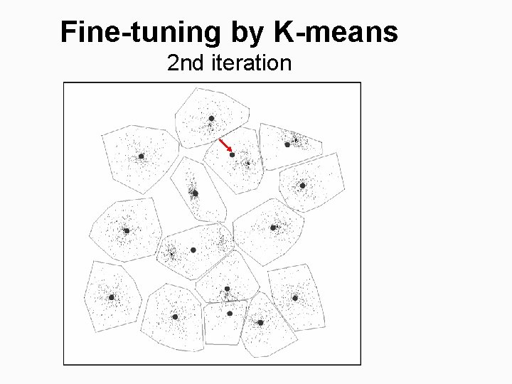
Fine-tuning by K-means 1 st iteration

Fine-tuning by K-means 2 nd iteration

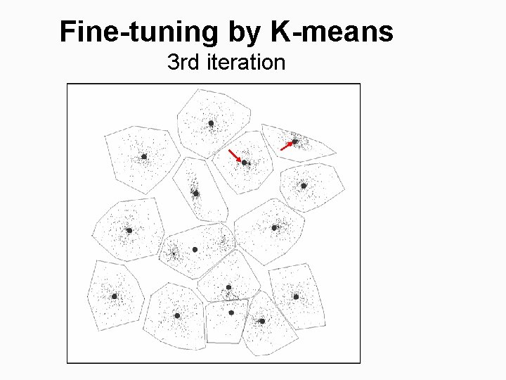
Fine-tuning by K-means 3 rd iteration

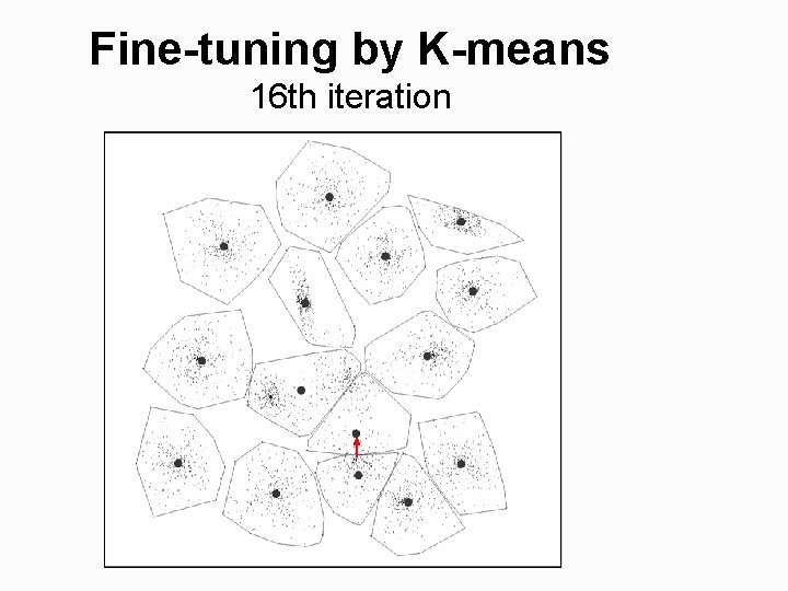
Fine-tuning by K-means 16 th iteration

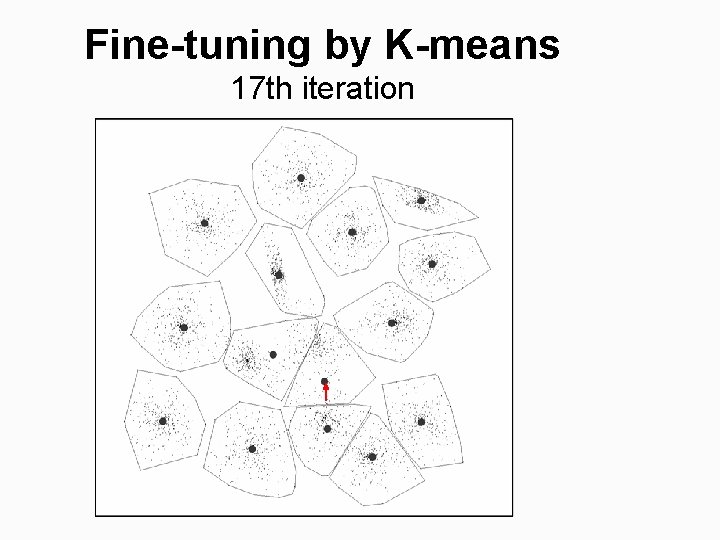
Fine-tuning by K-means 17 th iteration

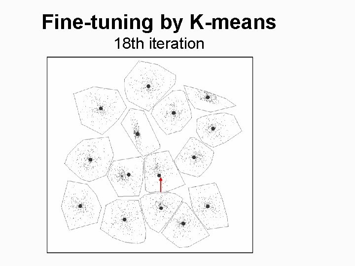
Fine-tuning by K-means 18 th iteration

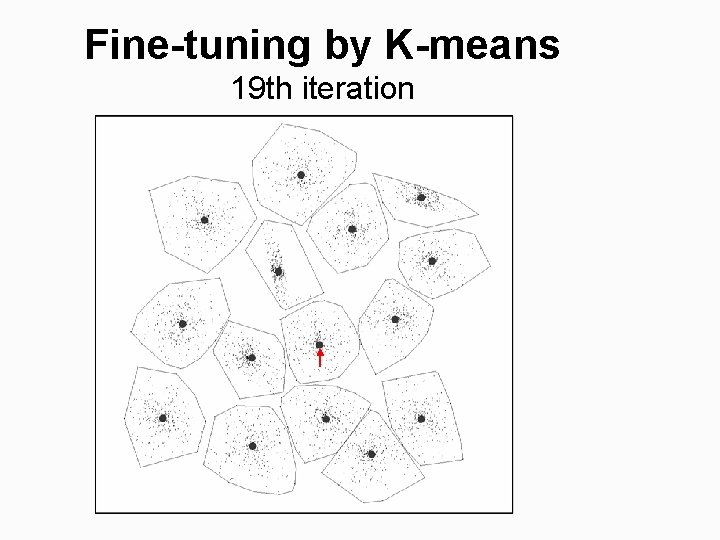
Fine-tuning by K-means 19 th iteration

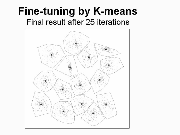
Fine-tuning by K-means Final result after 25 iterations

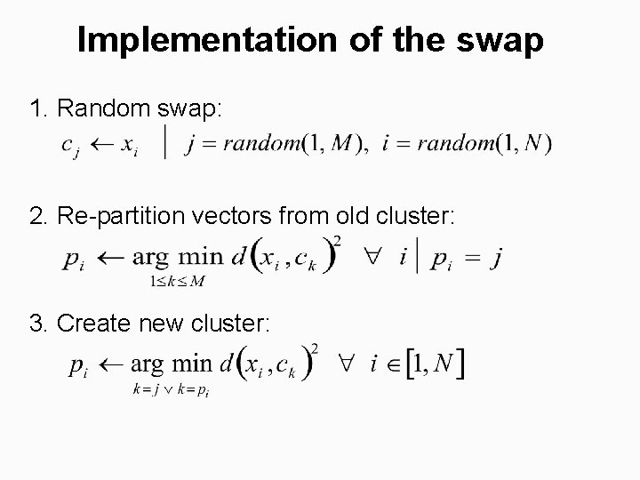
Implementation of the swap 1. Random swap: 2. Re-partition vectors from old cluster: 3. Create new cluster:

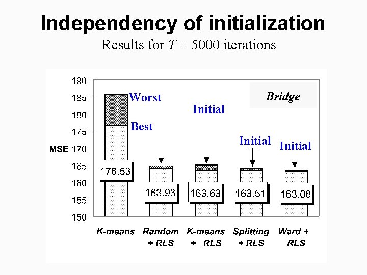
Independency of initialization Results for T = 5000 iterations Worst Initial Bridge Best Initial

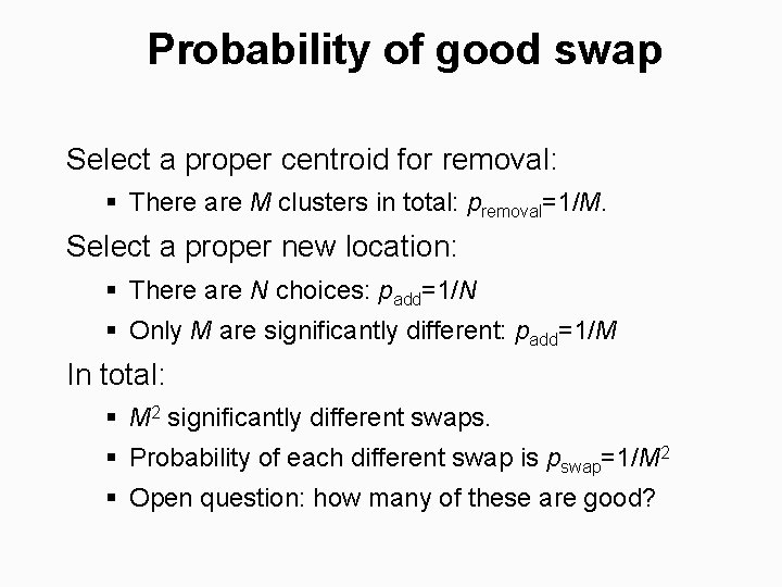
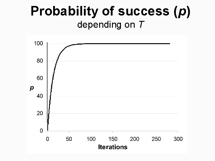
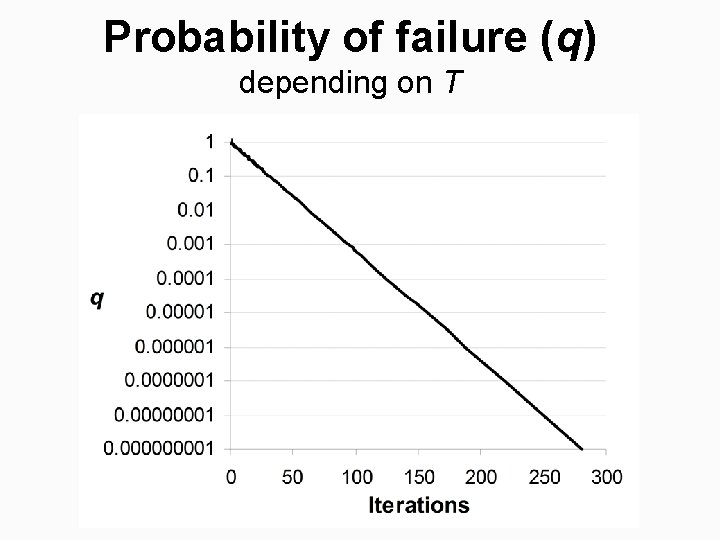
Probability of good swap Select a proper centroid for removal: § There are M clusters in total: premoval=1/M. Select a proper new location: § There are N choices: padd=1/N § Only M are significantly different: padd=1/M In total: § M 2 significantly different swaps. § Probability of each different swap is pswap=1/M 2 § Open question: how many of these are good?

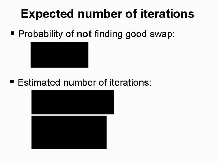
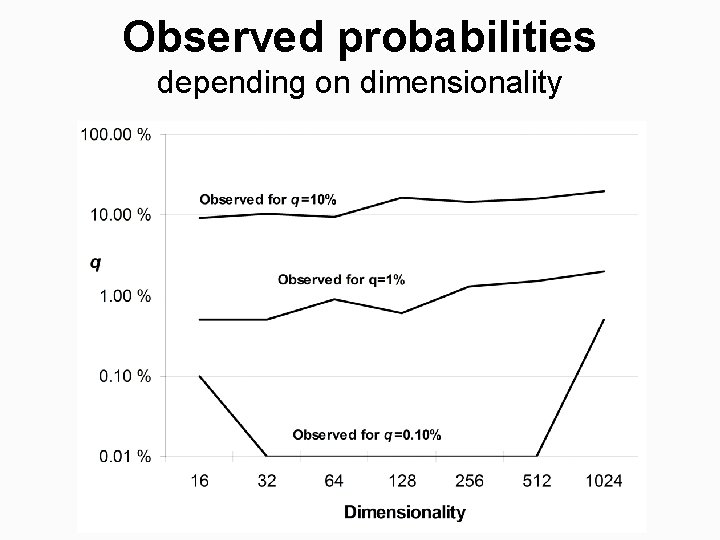
Expected number of iterations § Probability of not finding good swap: § Estimated number of iterations:

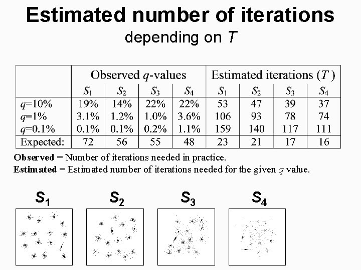
Estimated number of iterations depending on T Observed = Number of iterations needed in practice. Estimated = Estimated number of iterations needed for the given q value. S 1 S 2 S 3 S 4

Probability of success (p) depending on T

Probability of failure (q) depending on T

Observed probabilities depending on dimensionality

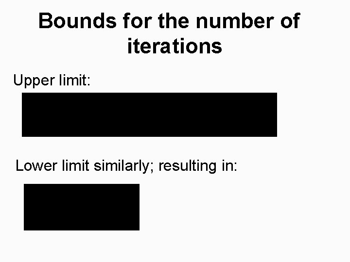
Bounds for the number of iterations Upper limit: Lower limit similarly; resulting in:

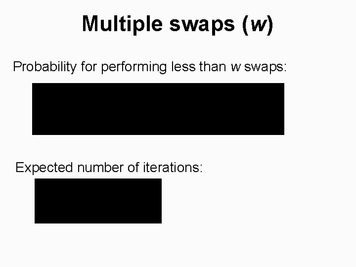
Multiple swaps (w) Probability for performing less than w swaps: Expected number of iterations:

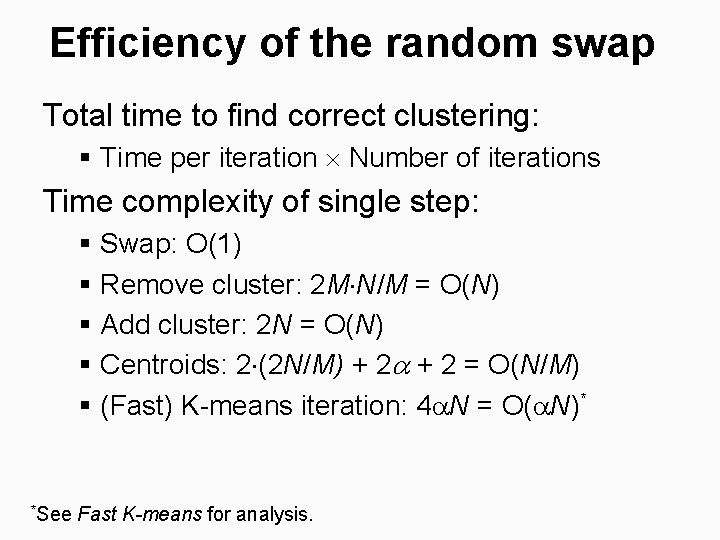
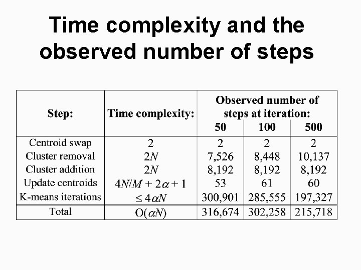
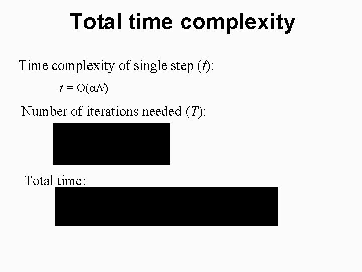
Efficiency of the random swap Total time to find correct clustering: § Time per iteration Number of iterations Time complexity of single step: § § § Swap: O(1) Remove cluster: 2 M N/M = O(N) Add cluster: 2 N = O(N) Centroids: 2 (2 N/M) + 2 = O(N/M) (Fast) K-means iteration: 4 N = O( N)* *See Fast K-means for analysis.

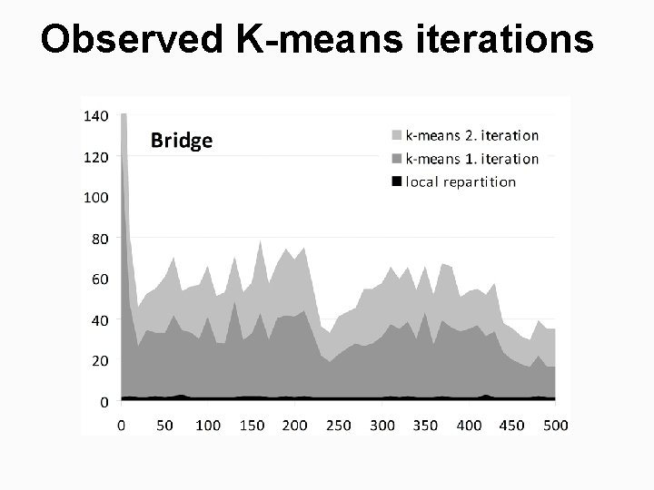
Observed K-means iterations

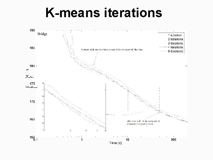
K-means iterations

Time complexity and the observed number of steps

Total time complexity Time complexity of single step (t): t = O(αN) Number of iterations needed (T): Total time:

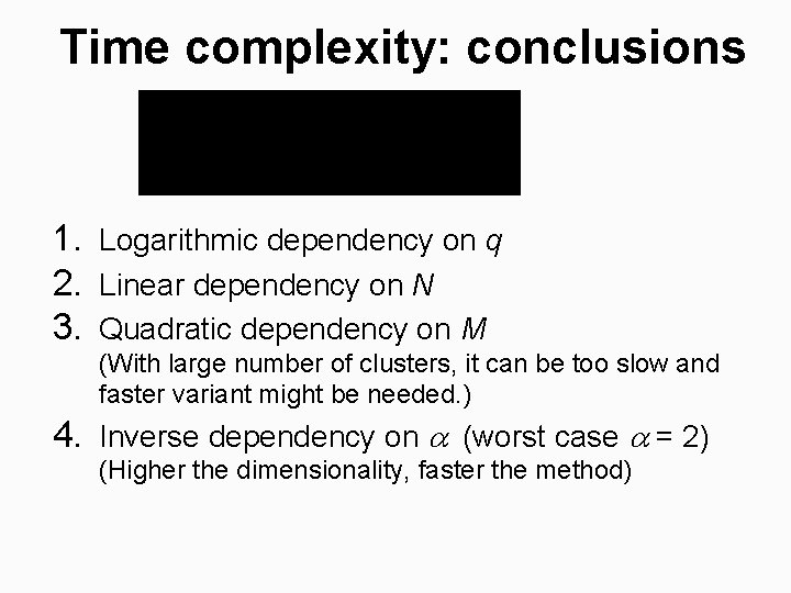
Time complexity: conclusions 1. Logarithmic dependency on q 2. Linear dependency on N 3. Quadratic dependency on M (With large number of clusters, it can be too slow and faster variant might be needed. ) 4. Inverse dependency on (worst case = 2) (Higher the dimensionality, faster the method)

References Random swap algorithm: • • P. Fränti and J. Kivijärvi, "Randomised local search algorithm for the clustering problem", Pattern Analysis and Applications, 3 (4), 358 -369, 2000. P. Fränti, J. Kivijärvi and O. Nevalainen, "Tabu search algorithm for codebook generation in VQ", Pattern Recognition, 31 (8), 1139‑ 1148, August 1998. Pseudo code: • http: //cs. uef. fi/sipu/ Efficiency of Random swap algorithm: • P. Fränti, O. Virmajoki and V. Hautamäki, “Efficiency of random swap based clustering", IAPR Int. Conf. on Pattern Recognition (ICPR’ 08), Tampa, FL, Dec 2008.

Part III: Efficient solution

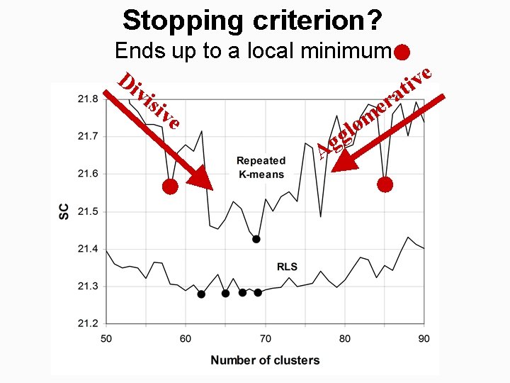
Stopping criterion? Ends up to a local minimum e Di v i t vis a r ive e m o l g Ag

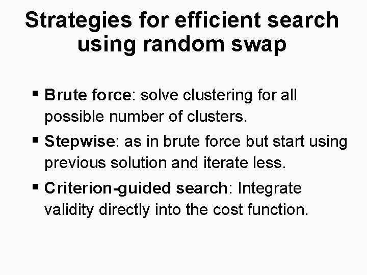
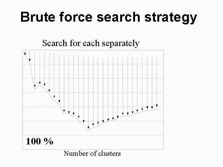
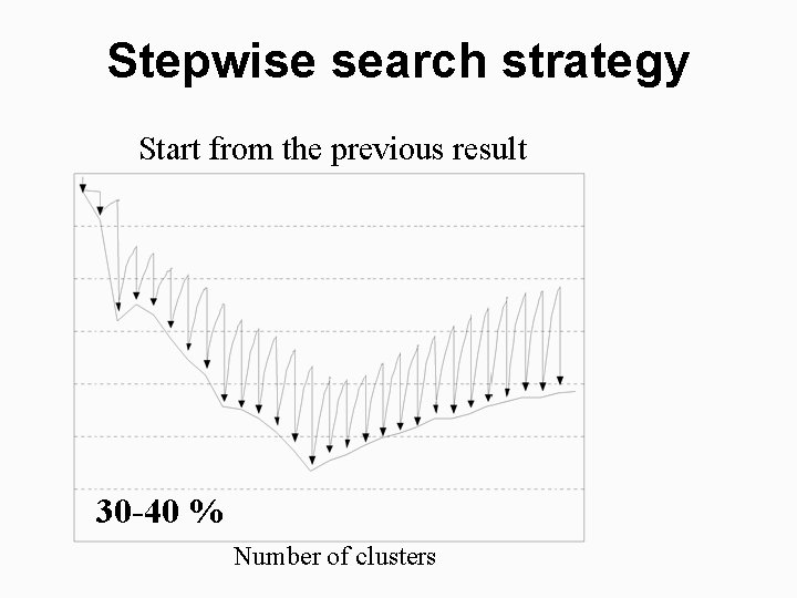
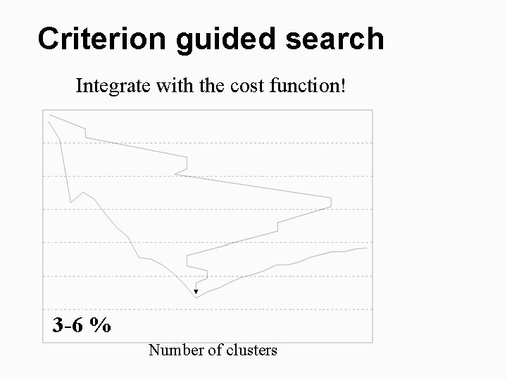
Strategies for efficient search using random swap § Brute force: solve clustering for all possible number of clusters. § Stepwise: as in brute force but start using previous solution and iterate less. § Criterion-guided search: Integrate validity directly into the cost function.

Brute force search strategy Search for each separately 100 % Number of clusters

Stepwise search strategy Start from the previous result 30 -40 % Number of clusters

Criterion guided search Integrate with the cost function! 3 -6 % Number of clusters

Conclusions Define the problem Cost function f. Measures the goodness of clusters, or alternatively (dis)similarity between two objects. Solve the problem Select the best algorithm for minimizing f Homework Number of clusters: Q. Zhao and P. Fränti, "WB-index: a sum-ofsquares based index for cluster validity", Data & Knowledge Engineering, 92: 77 -89, 2014. Validation: P. Fränti, M. Rezaei and Q. Zhao, "Centroid index: Cluster level similarity measure", Pattern Recognition, 47 (9), 3034 -3045, Sept. 2014.

Thank you Time for questions!