Extensions of Voronoi Diagrams Furthest Point Voronoi Diagram

Extensions of Voronoi Diagrams

Furthest Point Voronoi Diagram V-1(pi) : the set of point of the plane farther from pi than from any other site Vor-1(P) : the partition of the plane formed by the farthest point Voronoi regions, their edges, and vertices

Furthest Point Voronoi Region Construction of V-1(7) Property The farthest point Voronoi regions are convex

Furthest Point Voronoi Region Property If the farthest point Voronoi region of pi is non empty then pi is a vertex of the convex hull of P

Furthest Point Voronoi Region Property If pi is a vertex of convex hull of P then the farthest point Voronoi region of pi is non empty Property The farthest point Voronoi regions are unbounded Corollary The farthest point Voronoi edges and vertices form a tree V-1(4)

Farthest point Voronoi edges and vertices V-1(4) x V-1(1) V-1(7) V-1(2) edge : set of points equidistant from 2 sites and closer to all the other sites vertex : point equidistant from at least 3 sites and closer to all the other sites

Application: Smallest enclosing circle V-1(4) V-1(7) V-1(2)

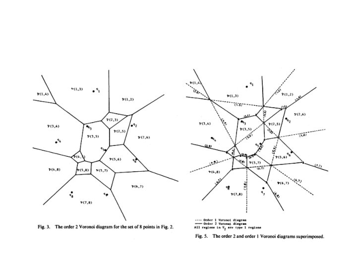
Higher Order Voronoi Diagrams (VD) kth order VD, Vk(S) • Vk(S) is a partition of the plane into regions such that points in each region have the same k closest sites.

3 th order Voronoi Diagram

• Let H be a subset of points of S. Let VS(H) denote the region such that for any point in the region, the |H| closest neighbors of S are the points of H. That is VS(H) = q ε H, q’ ε S-H h(q, q’) • Lee in 1982 presented an O(knlogn) algorithm where the kthe order Voronoi diagram is obtained from (k-1)th order Voronoi diagram. • The size of the kth order Voronoi diagram is O(k(n-k)).

Gabriel Graphs • Two points p and q are connected by an edge in the Gabriel graph whenever the disk having line segment pq as its diameter contains no other points from the given point set. • More generally, in any dimension, the Gabriel graph connects any two points forming the endpoints of the diameter of an empty sphere. Gabriel graphs are named after K. R. Gabriel, who introduced them in a paper with R. R. Sokal in 1969. • The Gabriel graph is a subgraph of the Delaunay triangulation; it can be found in linear time if the Delaunay triangulation is given (Matula and Sokal, 1980). The Gabriel graph contains as a subgraph the Euclidean minimum spanning tree and the nearest neighbor graph. • It is an instance of a beta-skeleton.

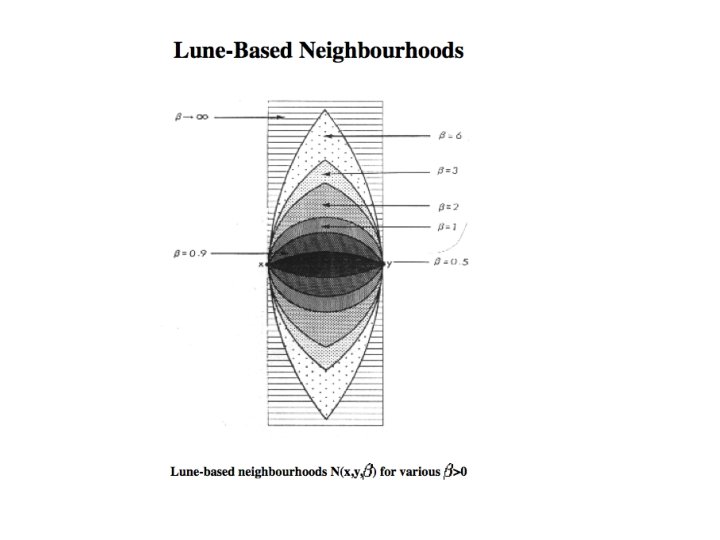
β-skeletons • Given a point set S, the β-Skeleton of S is the set of edges joining β -neighbors in S. • Given a point set S, two points x and y are β-neighbors in the set S if the region of influence of x and y, N(x, y, ) contains no point of S, other than x or y, in its interior. There are various kinds of definitions of N(x, y, ). One of them is called Lune. Based Neighborhoods. • First proposed by Kirkpatrick and Radke 1985, “A framework for computational morphology”

For β ≥ 1 We define N(x, y, β) to be the intersection of the two circles of radius d(x, y)/2 centered at the points (1 - β/2)x+(β/2)y and (β/2)x + (1 - β/2)y, respectively. β When β =1, N(x, y, β) corresponds exactly to the Gabriel neighborhood of x and y. When β =2, we get the ``relative neighborhood'' of the RNG. As β approaches infinity, the neighborhood of x and y approximates the infinite strip formed by translating the line segment (x, y) normal to itself. For β ε [0, 1] We define N(x, y, β) to be the intersection of the two circles of radius d(x, y)/(2β) passing through both x and y. When β =1, this is consistent with the definition above. As β approaches 0, N(x, y, β) approximates the line segment joining x and y. Thus, except in degenerate situations (three or more points collinear), all point pairs are β-neighbors under this scheme for β sufficiently small.

Alpha Shapes The space generated by point pairs that can be touched by an empty disc of radius alpha.

Alpha Hull • Definition: Let α be a sufficiently small but otherwise arbitrary positive real. The α-hull of S is the intersection all closed discs with radius 1/α that contain all the points of S.

Alpha Hull • Definition 1: Let α be a sufficiently small but otherwise arbitrary positive real. The α-hull of S is the intersection all closed discs with radius 1/α that contain all the points of S. The smallest possible value for 1/α is equal to the radius of the smallest enclosing circle.

Alpha Hull • Definition 2: For arbitrary negative real α, the αhull is defined as the intersection of all closed complements of discs (where these discs have radii -1/α) that contain all the points of S.

Alpha Hull • Definition 2: For arbitrary negative real α, the αhull is defined as the intersection of all closed complements of discs (where these discs have radii -1/α) that contain all the points of S. 0 -hull is the convex hull

Alpha Shapes • Definition 3: A point p in a set S is termed α-extreme in S if there exists a closed disc of radius 1/α (α +ve or α –ve) such that p lies on the boundary and it contains all the points of S. If for two α-extreme points p and q there exists a closed discs of radius 1/α (+ve or –ve) where both points lie on its boundary and which contains all other points, p and q are said to be α-neighbors.

Alpha Shapes • Definition 4: Given a set S of points in the plane and arbitrary α, the α-shape of S is the straight line graph whose vertices the α-extremes and whose edges connect the respective α-neighbors.

Alpha Shapes

Alpha Shapes Alpha Controls the desired level of detail.

-Shapes • DTf(S) : Delaunay triangulation of the farthest point Voronoi diagram of S. • DTc(S): Delaunay triangulation of the nearest neighbor Voronoi diagram of S. • Lemma: The α-shape of S is a subgraph of DTf(S) if α ≥ 0 and a subgraph of DTc(S) if α ≤ 0.

-Shapes • Theorem: For each Delaunay edge, e=(pi, pj), there exists min(e)>0 and max(e)>0 such that e -shape of S iff min(e) max(e). • Thus, every alpha-hull edge is in the Delaunay, and every Delaunay edge is in some alphashape.

-Shapes

-Shapes Running time: O(nlogn)

Papers • H. Edelsbrunner, D. G. Kirkpatrick and R. Seidel. On the shape of a set of points in the plane. IEEE Transactions on Information Theory, 1983. • H. Edelsbrunner and E. P. Mucke. Three dimensional alpha shapes, To. G 1994. • Kaspar Fischer, Introduction to alpha shapes.

Region aggregation • Triangulate between objects to be aggregated • Aggregate if: - the distance is small over a stretch - it reduces total boundary length

Region aggregation à la Jones et al. • More general: triangulate all and test where aggregation is good • Use constrained Delaunay triangulation

Constrained Delaunay Triangulations • S : Set of non-intersecting edges • CDT(S): A triangulation of the vertices with the following properties: – the edges are included in the triangulation – it is as close as possible by Delaunay Triangulation • The circumcircle through the vertices (say a, b and c) of each triangle does not contain – any endpoint of S that is visible from a, b and c.

Constrained Delaunay Triangulation • Delaunay: empty circle • Constrained Delaunay: empty circle but with given edges empty Needn’t be empty

Constrained Delaunay Triangulation • Delaunay: empty circle • Constrained Delaunay: empty circle but with given edges empty Needn’t be empty

Constrained Delaunay Triangulation

Constrained Delaunay Triangulation • Can be constructed in O(n log n) time (Chew, ’ 87) with sweep algorithm • Incremental also possible Usage: Places where aggregation is possible because objects are close enough and boundary length is reduced

Aggregation buildings • Flatten triangles in between • Reorient buildings • Test for possible conflicts Area preservation and more or less shape preservation Area preservation and more generalization

Shape change of natural objects • No restrictions on shape needed • Problem is self-coalescence, among which degree of detail

Shape change natural objects • Using triangulations: constrained Delaunay • Add triangles to polygon or remove them if that “improves” the shape