Exponential smoothing This is a widely used forecasting

Why is exponential smoothing so popular? üIt's easy—the exotic term notwithstanding. üData storage requirements

The basic algorithm (1) Where: • Lt is the forecast for the current period;

Equation (1) can be written as follows: New Forecast = (New Data) + (1

Exponential smoothing is weighted moving average process To demonstrate, let Substitute (2) into (1):

But notice that: (4) Substitute (4) into (3) to obtain: If we continue to

Notice that are the weights attached to past values of X. Since < 1,

You don’t have to go through this recursive process each time you do a

Selecting the smoothing constant ( ) • The range of possible values is zero

We will now forecast sales of liquor and floor covering using this technique. We

Summary Statistics Beer, Wine, Liquor Mean Standard Error Median Mode Standard Deviation Sample Variance

Beer, Wine, Liquor = 0. 1904 Parts, Tires, etc. = 0. 099 The ratio

Selecting the smoothing constant • Pricey time series forecasting software, such as EViews, use

Auto Parts, Accessories, and Tires (Alpha =. 69) Year 2006 2006 2007 2007 Month

Beer, Wine, and Liquor (Alpha =. 1280) Year 2006 2006 2007 2007 Month 7

Forecasts for August, 2007 Remember our basic algorithm Hence to parts, accessories, and tire

Slides: 19

Download presentation

Exponential smoothing This is a widely used forecasting technique in retailing, even though it has not proven to be especially accurate.

Why is exponential smoothing so popular? üIt's easy—the exotic term notwithstanding. üData storage requirements are minimal (even though this is not the problem it once was due to plunging memory prices). üIt is very cost effective when forecasts must be made for a large number of items--hence it has extensive use in retailing.

The basic algorithm (1) Where: • Lt is the forecast for the current period; • Xt is the most recent observation of the time series variable —such as, for example, sales last month of part #000897 • Lt-1 is the most recent forecast; and • is the smoothing constant, where 0 < < 1

Equation (1) can be written as follows: New Forecast = (New Data) + (1 - )Most Recent Forecast

Exponential smoothing is weighted moving average process To demonstrate, let Substitute (2) into (1): (3)

But notice that: (4) Substitute (4) into (3) to obtain: If we continue to substitute recursively, we get:

Notice that are the weights attached to past values of X. Since < 1, the weights attached to earlier or more remote observations of X are diminishing.

You don’t have to go through this recursive process each time you do a forecast. The process is summarized in the most recent forecast.

Selecting the smoothing constant ( ) • The range of possible values is zero and one. Sales of part #56 • If you select a value of close to 1, that means you are attaching a large weight to the most recent observation. This is not indicated if your series is very erratic (swings widely from period to period). For example, suppose you were forecasting the demand for part #56 in month t. If you attached too much weight to the observation for t-1, you will have a large forecast error for month t. t-2 t-1 t Month

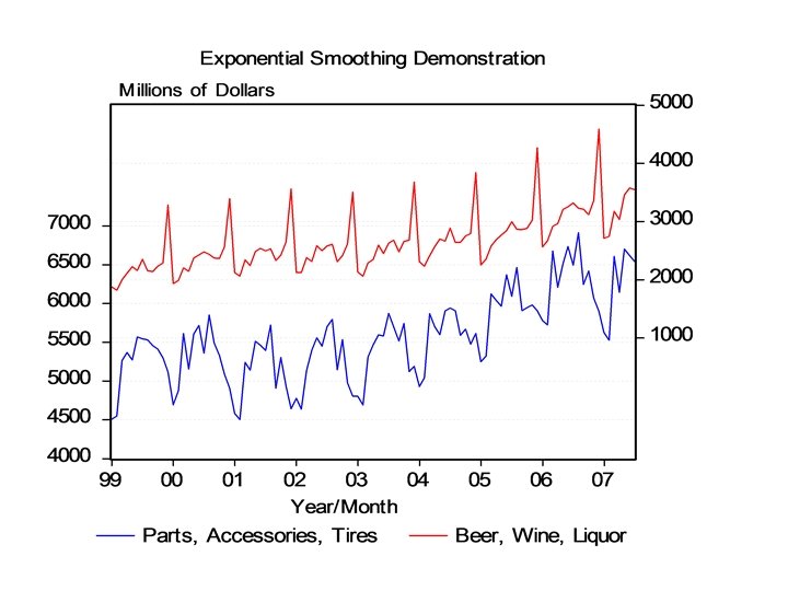
We will now forecast sales of liquor and floor covering using this technique. We have monthly data for each variable beginning in January 1999 and running through July of 2007.

Summary Statistics Beer, Wine, Liquor Mean Standard Error Median Mode Standard Deviation Sample Variance Kurtosis Skewness Range Minimum Maximum Sum Count Parts, Accessories, Tires 2653. 35922 49. 798155 2567 2232 Mean Standard Error Median Mode 5568. 1068 54. 5247066 5546 5613 505. 396076 255425. 193 1. 88359717 1. 19777269 2770 1818 4588 273296 103 Standard Deviation Sample Variance Kurtosis Skewness Range Minimum Maximum Sum Count 553. 365335 306213. 194 -0. 2735442 0. 23599223 2411 4503 6914 573515 103

Beer, Wine, Liquor = 0. 1904 Parts, Tires, etc. = 0. 099 The ratio of the standard deviation to the mean gives us a nice measure of the amplitude or volatility of a series month-to-month (or day-to-day, quarter-toquarter, as the case may be).

Selecting the smoothing constant • Pricey time series forecasting software, such as EViews, use an algorithm to select the value of the smoothing constant that minimizes mean square error for in-sample forecasts. • If you lack this software, you can use a trial and error process.

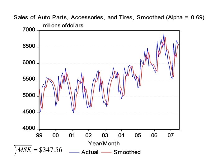
Auto Parts, Accessories, and Tires (Alpha =. 69) Year 2006 2006 2007 2007 Month 7 8 9 10 11 12 1 2 3 4 5 6 7 Actual 6493 6914 6245 6419 6072 5900 5628 5526 6608 6144 6702 6619 6538 Smoothed 6642. 08 6539. 21 6797. 82 6416. 37 6418. 19 6179. 32 5986. 59 5739. 16 5592. 08 6293. 06 6190. 21 6543. 34 6595. 55

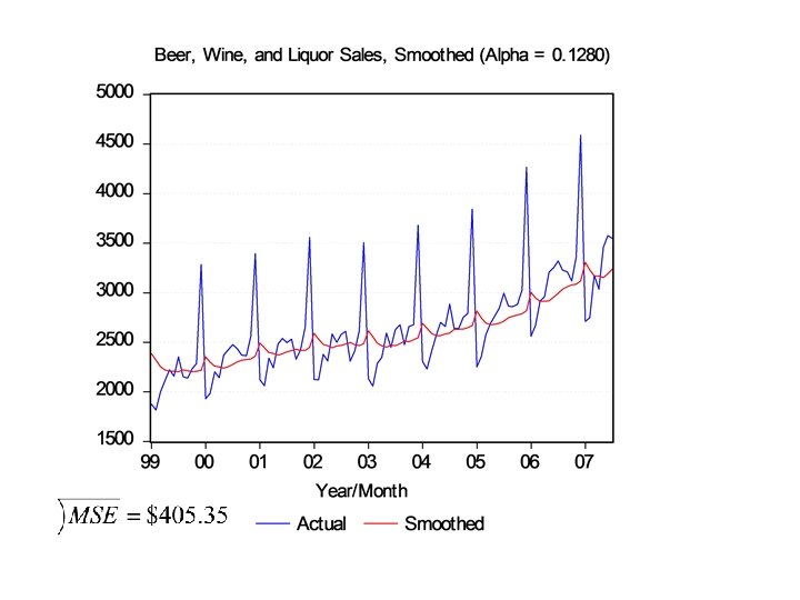
Beer, Wine, and Liquor (Alpha =. 1280) Year 2006 2006 2007 2007 Month 7 8 9 10 11 12 1 2 3 4 5 6 7 Actual 3322 3228 3212 3120 3359 4588 2710 2748 3176 3037 3459 3578 3547 Smoothed 2994. 10 3036. 07 3060. 64 3080. 01 3085. 13 3120. 19 3308. 08 3231. 52 3169. 63 3170. 44 3153. 36 3192. 48 3241. 83

Forecasts for August, 2007 Remember our basic algorithm Hence to parts, accessories, and tire sales (PAT) for August, 2007: To forecast beer, wine, and liquor sales (BWL):