Exponential Smoothing Exponential Smoothing Methods This method provides

Exponential Smoothing

Exponential Smoothing Methods • This method provides an exponentially weighted moving average of all previously observed values. • Appropriate for data with no predictable upward or downward trend. • The aim is to estimate the current level and use it as a forecast of future value.

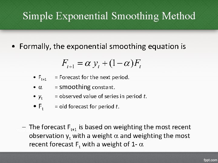
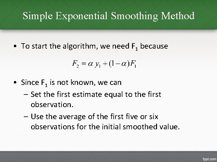
Simple Exponential Smoothing Method • Formally, the exponential smoothing equation is • Ft+1 = Forecast for the next period. • • yt = smoothing constant. = observed value of series in period t. • Ft = old forecast for period t. – The forecast Ft+1 is based on weighting the most recent observation yt with a weight and weighting the most recent forecast Ft with a weight of 1 -

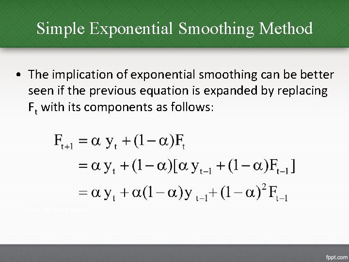
Simple Exponential Smoothing Method • The implication of exponential smoothing can be better seen if the previous equation is expanded by replacing Ft with its components as follows:

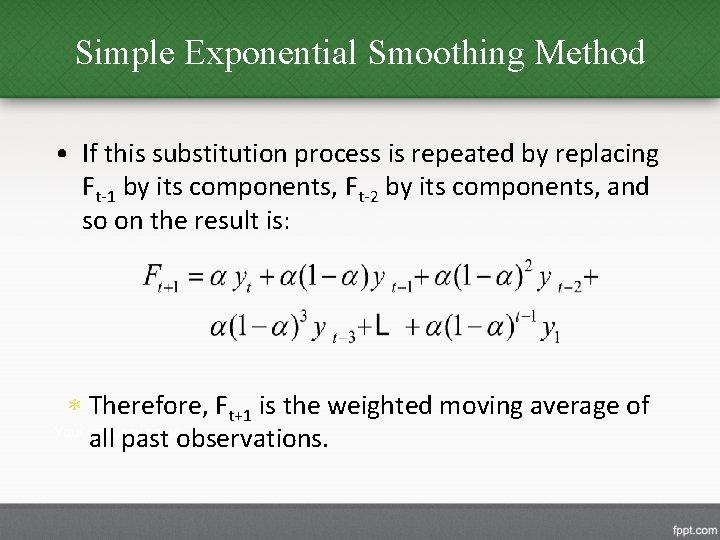
Simple Exponential Smoothing Method • If this substitution process is repeated by replacing Ft-1 by its components, Ft-2 by its components, and so on the result is: Therefore, Ft+1 is the weighted moving average of all past observations.

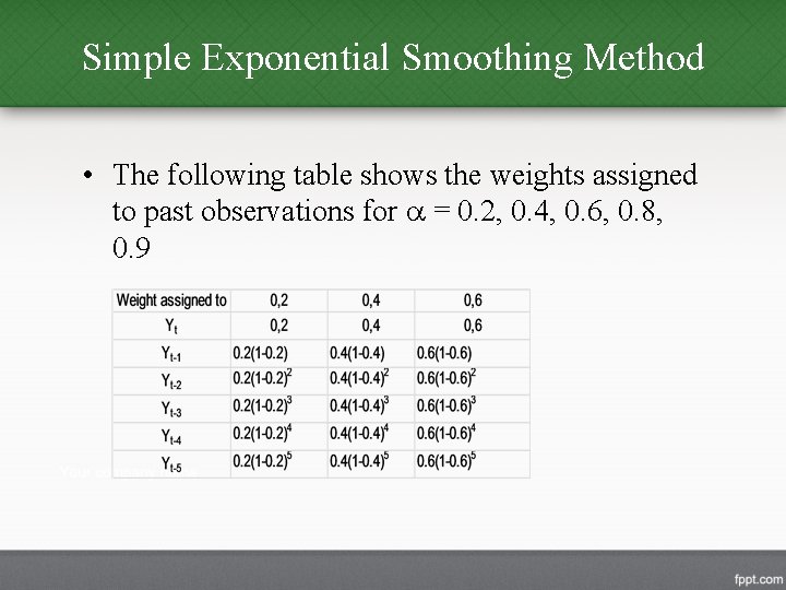
Simple Exponential Smoothing Method • The following table shows the weights assigned to past observations for = 0. 2, 0. 4, 0. 6, 0. 8, 0. 9

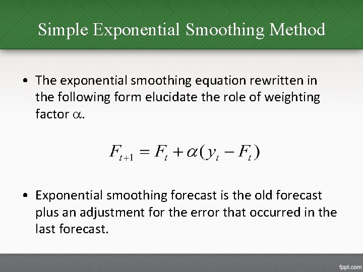
Simple Exponential Smoothing Method • The exponential smoothing equation rewritten in the following form elucidate the role of weighting factor . • Exponential smoothing forecast is the old forecast plus an adjustment for the error that occurred in the last forecast.

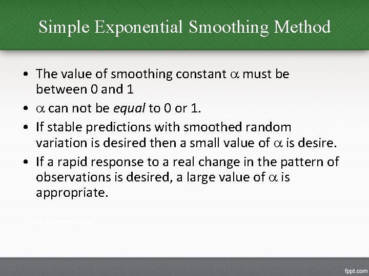
Simple Exponential Smoothing Method • The value of smoothing constant must be between 0 and 1 • can not be equal to 0 or 1. • If stable predictions with smoothed random variation is desired then a small value of is desire. • If a rapid response to a real change in the pattern of observations is desired, a large value of is appropriate.

Simple Exponential Smoothing Method • To estimate , Forecasts are computed for equal to. 1, . 2, . 3, …, . 9 and the sum of squared forecast error is computed for each. • The value of with the smallest RMSE is chosen for use in producing the future forecasts.

Simple Exponential Smoothing Method • To start the algorithm, we need F 1 because • Since F 1 is not known, we can – Set the first estimate equal to the first observation. – Use the average of the first five or six observations for the initial smoothed value.

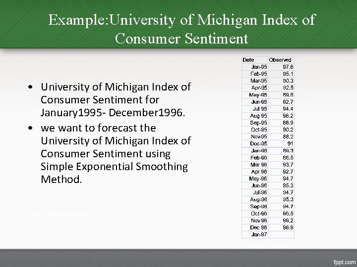
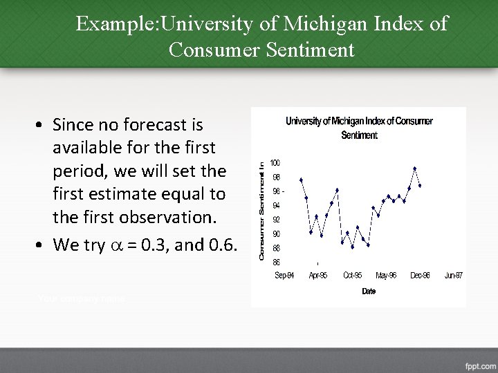
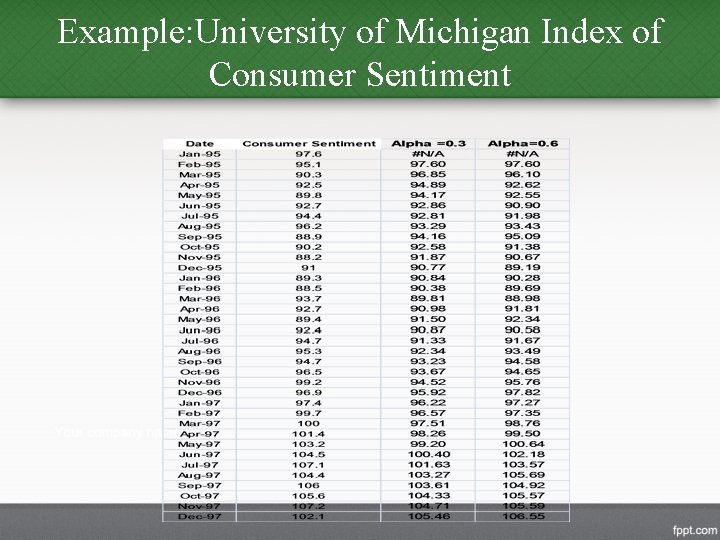
Example: University of Michigan Index of Consumer Sentiment • University of Michigan Index of Consumer Sentiment for January 1995 - December 1996. • we want to forecast the University of Michigan Index of Consumer Sentiment using Simple Exponential Smoothing Method.

Example: University of Michigan Index of Consumer Sentiment • Since no forecast is available for the first period, we will set the first estimate equal to the first observation. • We try = 0. 3, and 0. 6.

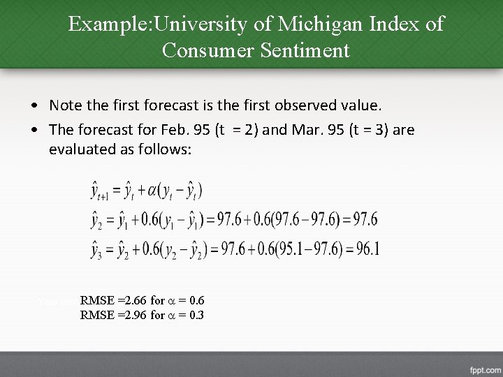
Example: University of Michigan Index of Consumer Sentiment • Note the first forecast is the first observed value. • The forecast for Feb. 95 (t = 2) and Mar. 95 (t = 3) are evaluated as follows: RMSE =2. 66 for = 0. 6 RMSE =2. 96 for = 0. 3

Example: University of Michigan Index of Consumer Sentiment

Holt’s Exponential smoothing • Holt’s two parameter exponential smoothing method is an extension of simple exponential smoothing. • It adds a growth factor (or trend factor) to the smoothing equation as a way of adjusting for the trend.

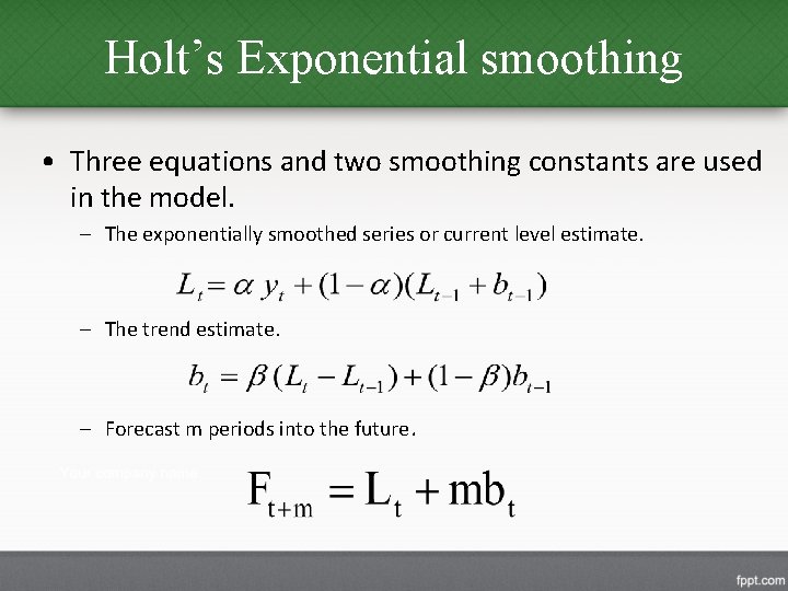
Holt’s Exponential smoothing • Three equations and two smoothing constants are used in the model. – The exponentially smoothed series or current level estimate. – The trend estimate. – Forecast m periods into the future.

Holt’s Exponential smoothing – Lt – – yt – – bt – m = Estimate of the level of the series at time t = smoothing constant for the data. = new observation or actual value of series in period t. = smoothing constant for trend estimate = estimate of the slope of the series at time t = periods to be forecast into the future.

Holt’s Exponential smoothing • The weight and can be selected subjectively or by minimizing a measure of forecast error such as RMSE. • Large weights result in more rapid changes in the component. • Small weights result in less rapid changes.

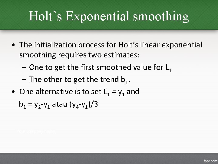
Holt’s Exponential smoothing • The initialization process for Holt’s linear exponential smoothing requires two estimates: – One to get the first smoothed value for L 1 – The other to get the trend b 1. • One alternative is to set L 1 = y 1 and b 1 = y 2 -y 1 atau (y 4 -y 1)/3

Example: Quarterly sales of saws for Acme tool company • The following table shows the sales of saws for the Acme tool Company. • These are quarterly sales From 1994 through 2000.

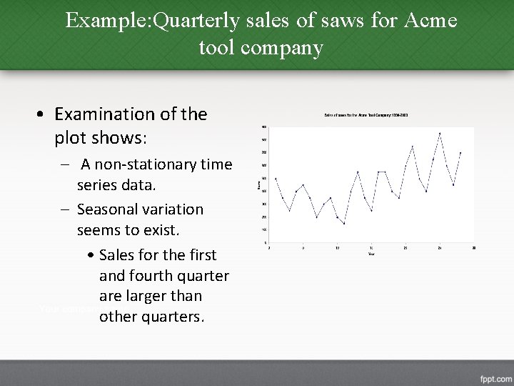
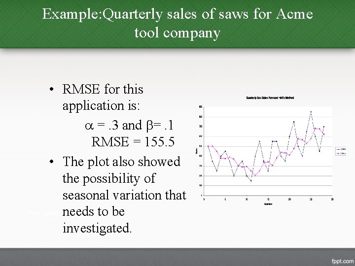
Example: Quarterly sales of saws for Acme tool company • Examination of the plot shows: – A non-stationary time series data. – Seasonal variation seems to exist. • Sales for the first and fourth quarter are larger than other quarters.

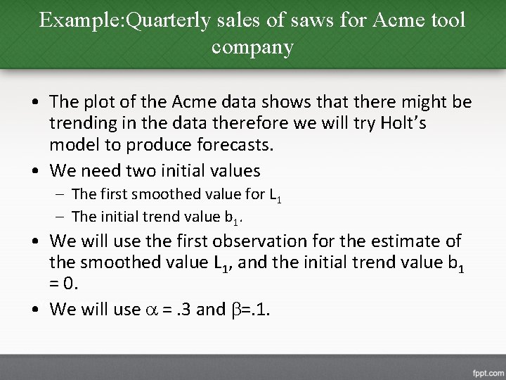
Example: Quarterly sales of saws for Acme tool company • The plot of the Acme data shows that there might be trending in the data therefore we will try Holt’s model to produce forecasts. • We need two initial values – The first smoothed value for L 1 – The initial trend value b 1. • We will use the first observation for the estimate of the smoothed value L 1, and the initial trend value b 1 = 0. • We will use =. 3 and =. 1.

Example: Quarterly sales of saws for Acme tool company

Example: Quarterly sales of saws for Acme tool company • RMSE for this application is: =. 3 and =. 1 RMSE = 155. 5 • The plot also showed the possibility of seasonal variation that needs to be investigated.

Winter’s Exponential Smoothing • Winter’s exponential smoothing model is the second extension of the basic Exponential smoothing model. • It is used for data that exhibit both trend and seasonality. • It is a three parameter model that is an extension of Holt’s method. • An additional equation adjusts the model for the seasonal component.

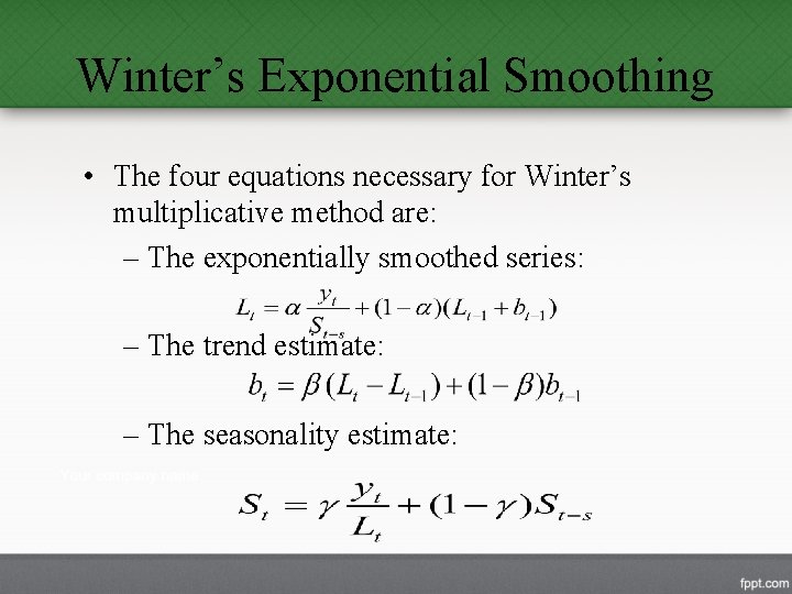
Winter’s Exponential Smoothing • The four equations necessary for Winter’s multiplicative method are: – The exponentially smoothed series: – The trend estimate: – The seasonality estimate:

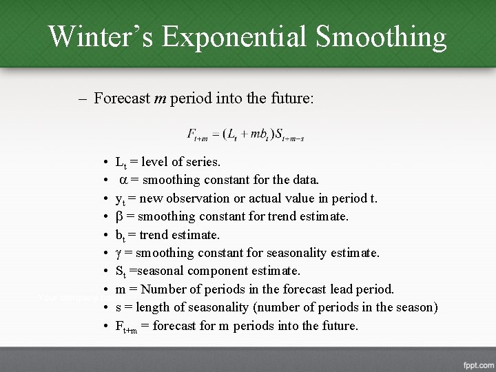
Winter’s Exponential Smoothing – Forecast m period into the future: • • • Lt = level of series. = smoothing constant for the data. yt = new observation or actual value in period t. = smoothing constant for trend estimate. bt = trend estimate. = smoothing constant for seasonality estimate. St =seasonal component estimate. m = Number of periods in the forecast lead period. s = length of seasonality (number of periods in the season) Ft+m = forecast for m periods into the future.

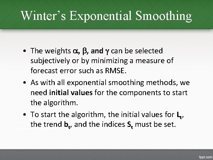
Winter’s Exponential Smoothing • The weights , , and can be selected subjectively or by minimizing a measure of forecast error such as RMSE. • As with all exponential smoothing methods, we need initial values for the components to start the algorithm. • To start the algorithm, the initial values for Lt, the trend bt, and the indices St must be set.

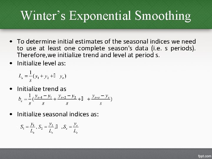
Winter’s Exponential Smoothing • To determine initial estimates of the seasonal indices we need to use at least one complete season's data (i. e. s periods). Therefore, we initialize trend and level at period s. • Initialize level as: • Initialize trend as • Initialize seasonal indices as:

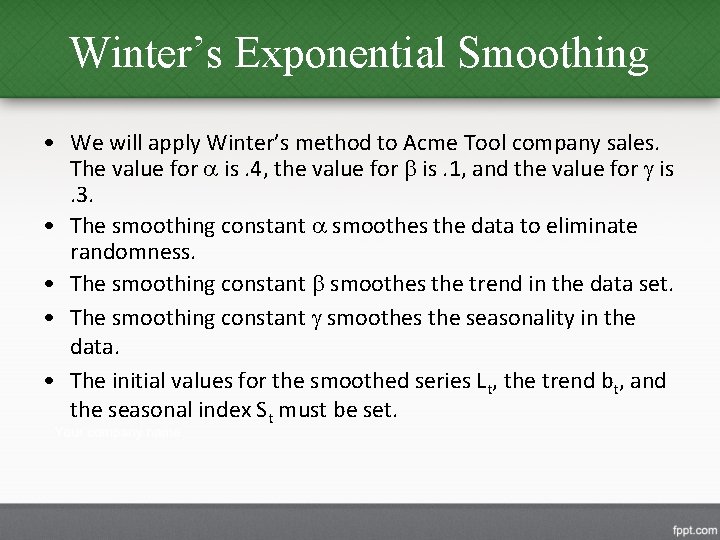
Winter’s Exponential Smoothing • We will apply Winter’s method to Acme Tool company sales. The value for is. 4, the value for is. 1, and the value for is. 3. • The smoothing constant smoothes the data to eliminate randomness. • The smoothing constant smoothes the trend in the data set. • The smoothing constant smoothes the seasonality in the data. • The initial values for the smoothed series Lt, the trend bt, and the seasonal index St must be set.

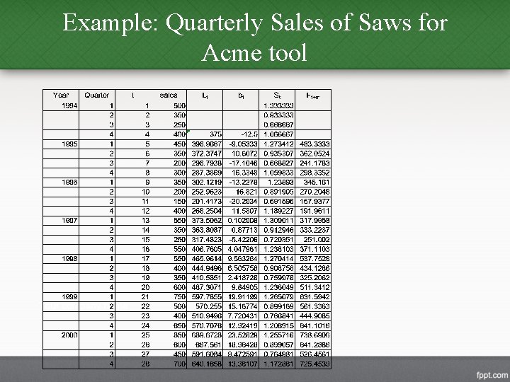
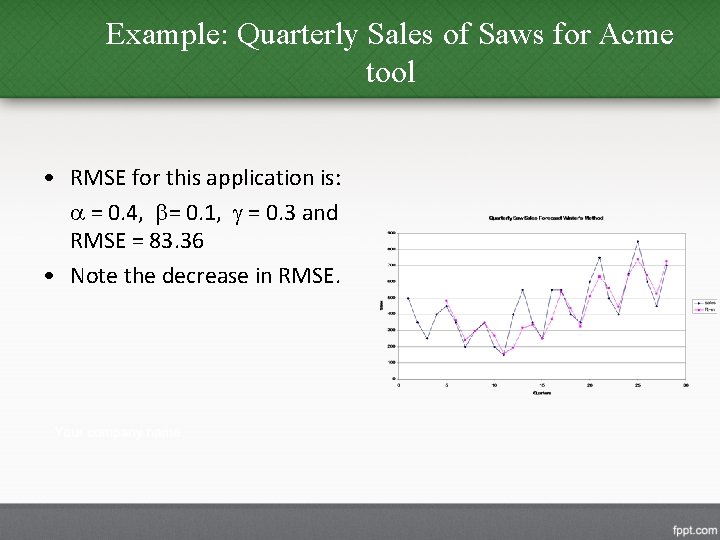
Example: Quarterly Sales of Saws for Acme tool

Example: Quarterly Sales of Saws for Acme tool • RMSE for this application is: = 0. 4, = 0. 1, = 0. 3 and RMSE = 83. 36 • Note the decrease in RMSE.

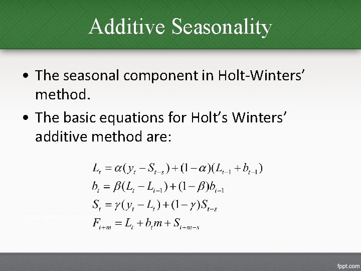
Additive Seasonality • The seasonal component in Holt-Winters’ method. • The basic equations for Holt’s Winters’ additive method are:

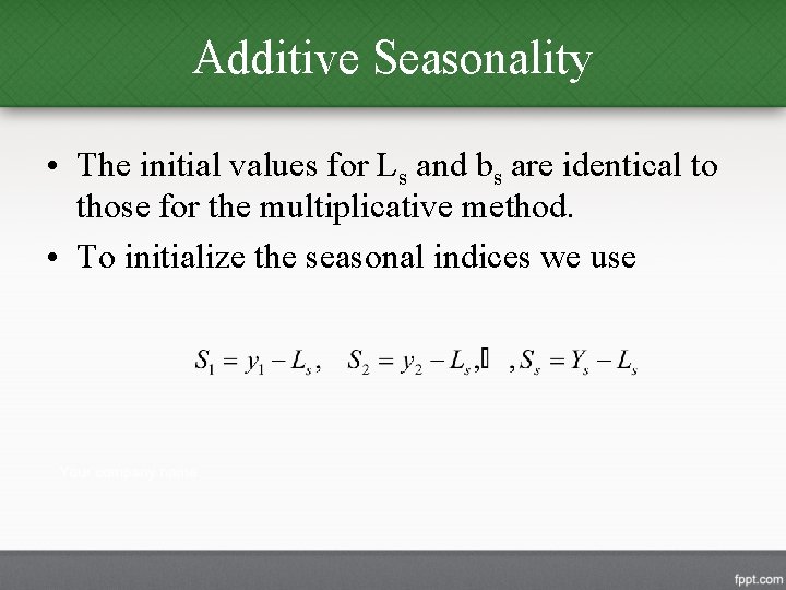
Additive Seasonality • The initial values for Ls and bs are identical to those for the multiplicative method. • To initialize the seasonal indices we use