Exploring the Shape of the DoseResponse Function Outline

Exploring the Shape of the Dose-Response Function

Outline · Traditional approach to dose-response analysis · The “step function” · Alternative: “Flexible” regression line · Spline regression · Examples: logistic/linear/Cox

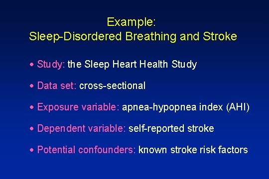
Example: Sleep-Disordered Breathing and Stroke · Study: the Sleep Heart Health Study · Data set: cross-sectional · Exposure variable: apnea-hypopnea index (AHI) · Dependent variable: self-reported stroke · Potential confounders: known stroke risk factors

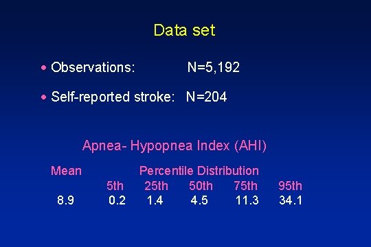
Data set · Observations: N=5, 192 · Self-reported stroke: N=204 Apnea- Hypopnea Index (AHI) Mean 8. 9 5 th 0. 2 Percentile Distribution 25 th 50 th 75 th 1. 4 4. 5 11. 3 95 th 34. 1

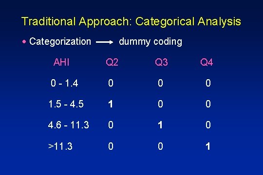
Traditional Approach: Categorical Analysis · Categorization dummy coding AHI Q 2 Q 3 Q 4 0 - 1. 4 0 0 0 1. 5 - 4. 5 1 0 0 4. 6 - 11. 3 0 1 0 >11. 3 0 0 1

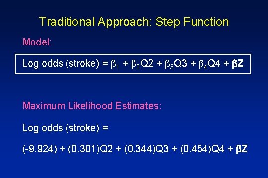
Traditional Approach: Step Function Model: Log odds (stroke) = 1 + 2 Q 2 + 3 Q 3 + 4 Q 4 + Z Maximum Likelihood Estimates: Log odds (stroke) = (-9. 924) + (0. 301)Q 2 + (0. 344)Q 3 + (0. 454)Q 4 + Z

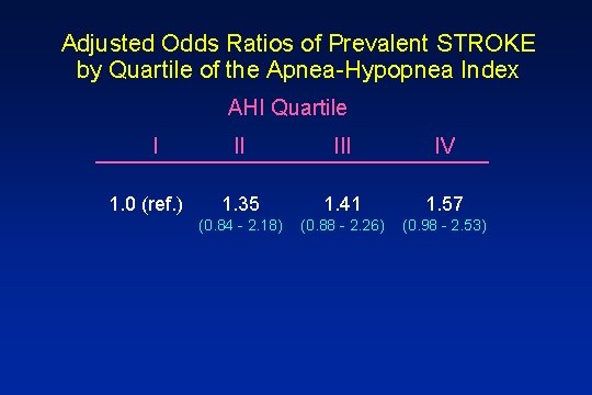
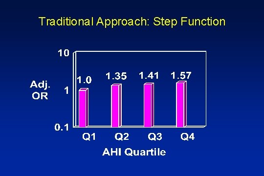
Adjusted Odds Ratios of Prevalent STROKE by Quartile of the Apnea-Hypopnea Index AHI Quartile I 1. 0 (ref. ) II IV 1. 35 1. 41 1. 57 (0. 84 - 2. 18) (0. 88 - 2. 26) (0. 98 - 2. 53)

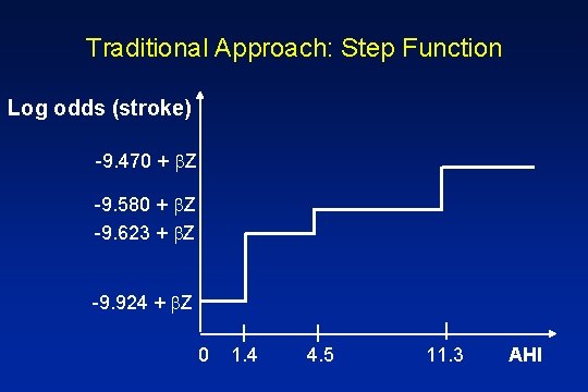
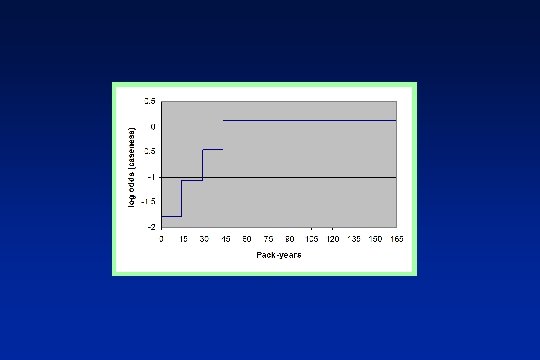
Traditional Approach: Step Function

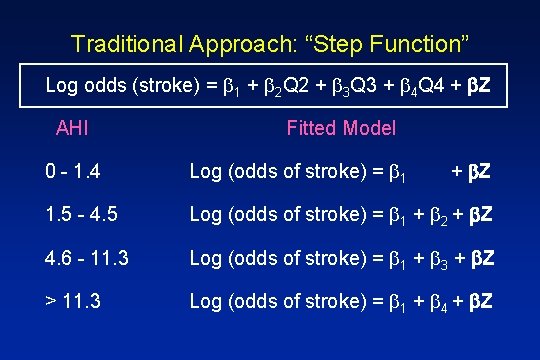
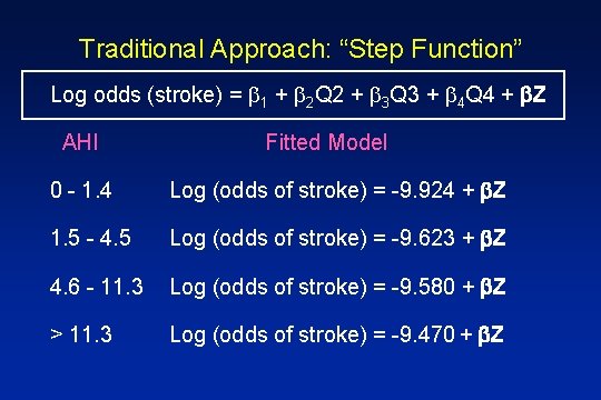
Traditional Approach: “Step Function” Log odds (stroke) = 1 + 2 Q 2 + 3 Q 3 + 4 Q 4 + Z AHI Fitted Model 0 - 1. 4 Log (odds of stroke) = 1 + Z 1. 5 - 4. 5 Log (odds of stroke) = 1 + 2 + Z 4. 6 - 11. 3 Log (odds of stroke) = 1 + 3 + Z > 11. 3 Log (odds of stroke) = 1 + 4 + Z

Traditional Approach: “Step Function” Log odds (stroke) = 1 + 2 Q 2 + 3 Q 3 + 4 Q 4 + Z AHI Fitted Model 0 - 1. 4 Log (odds of stroke) = -9. 924 + Z 1. 5 - 4. 5 Log (odds of stroke) = -9. 623 + Z 4. 6 - 11. 3 Log (odds of stroke) = -9. 580 + Z > 11. 3 Log (odds of stroke) = -9. 470 + Z

Traditional Approach: Step Function Log odds (stroke) -9. 470 + Z -9. 580 + Z -9. 623 + Z -9. 924 + Z 0 1. 4 4. 5 11. 3 AHI

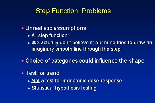
Step Function: Problems · Unrealistic assumptions A “step function” · We actually don’t believe it; our mind tries to draw an imaginary smooth line through the step · · Choice of categories could influence the shape · Test for trend Not a test for monotonic dose-response · Statistical hypothesis testing ·

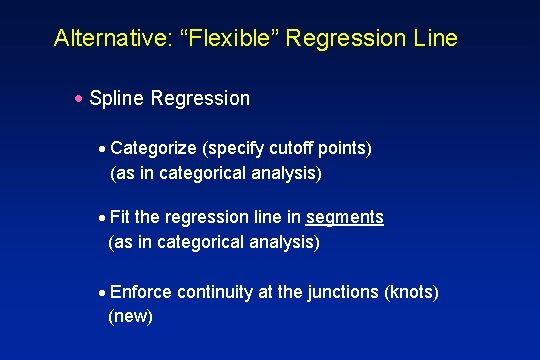
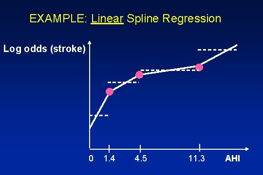
Alternative: “Flexible” Regression Line · Spline Regression · Categorize (specify cutoff points) (as in categorical analysis) · Fit the regression line in segments (as in categorical analysis) · Enforce continuity at the junctions (knots) (new)

EXAMPLE: Linear Spline Regression Log odds (stroke) 0 1. 4 4. 5 11. 3 AHI

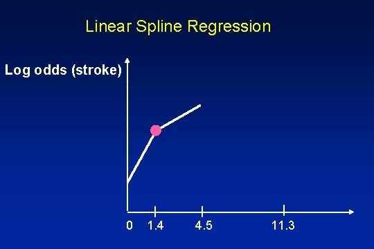
Linear Spline Regression Log odds (stroke) 0 1. 4 4. 5 11. 3

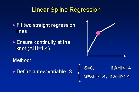
Linear Spline Regression · Fit two straight regression lines · Ensure continuity at the knot (AHI=1. 4) Method: · Define a new variable, S S=0, if AHI<1. 4 S=AHI-1. 4, if AHI>1. 4

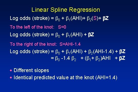
Linear Spline Regression Log odds (stroke) = 0 + 1(AHI)+ 2(S)+ Z To the left of the knot: S=0 Log odds (stroke) = 0 + 1(AHI) + Z To the right of the knot: S=AHI-1. 4 Log odds (stroke) = 0 + 1(AHI) + 2(AHI-1. 4) + Z = 0 -1. 4 2 + ( 1+ 2)AHI + Z · Different slopes · Identical predicted value at the knot (AHI=1. 4)

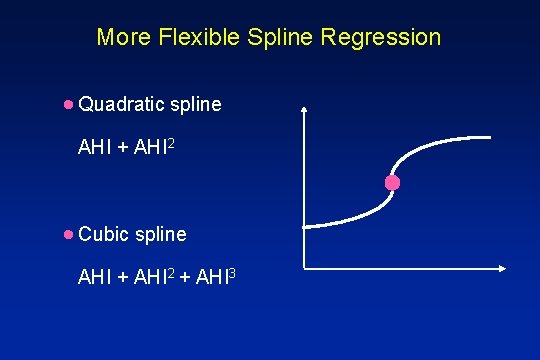
More Flexible Spline Regression · Quadratic spline AHI + AHI 2 · Cubic spline AHI + AHI 2 + AHI 3

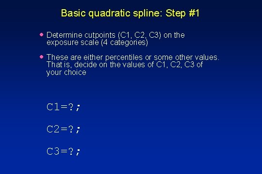
Basic quadratic spline: Step #1 · Determine cutpoints (C 1, C 2, C 3) on the exposure scale (4 categories) · These are either percentiles or some other values. That is, decide on the values of C 1, C 2, C 3 of your choice C 1=? ; C 2=? ; C 3=? ;

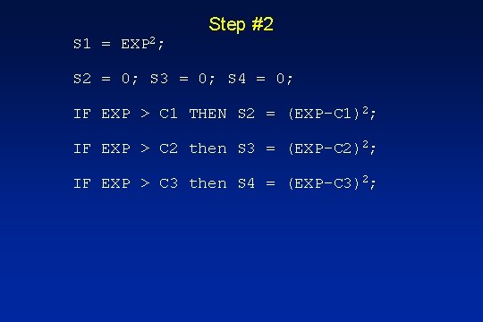
Step #2 S 1 = EXP 2; S 2 = 0; S 3 = 0; S 4 = 0; IF EXP > C 1 THEN S 2 = (EXP-C 1)2; IF EXP > C 2 then S 3 = (EXP-C 2)2; IF EXP > C 3 then S 4 = (EXP-C 3)2;

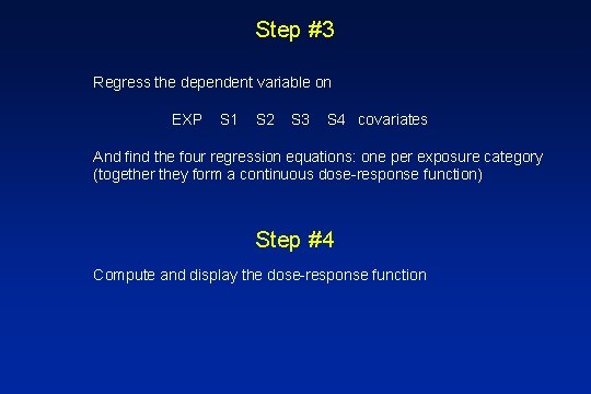
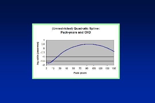
Step #3 Regress the dependent variable on EXP S 1 S 2 S 3 S 4 covariates And find the four regression equations: one per exposure category (together they form a continuous dose-response function) Step #4 Compute and display the dose-response function

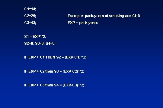
C 1=14; C 2=29; Example: pack-years of smoking and CHD C 3=43; EXP = pack-years S 1 = EXP**2; S 2=0; S 3=0; S 4=0; IF EXP > C 1 THEN S 2 = (EXP-C 1)**2; IF EXP > C 2 then S 3 = (EXP-C 2)**2; IF EXP > C 3 then S 4 = (EXP-C 3)**2;

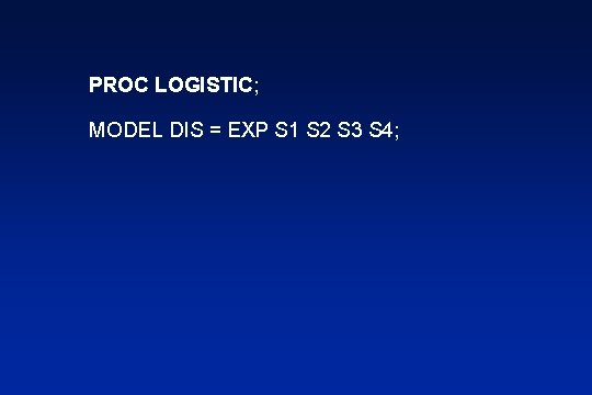
PROC LOGISTIC; MODEL DIS = EXP S 1 S 2 S 3 S 4;

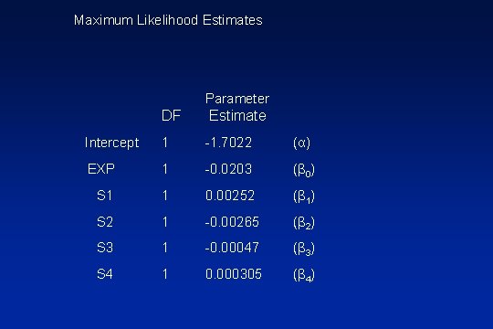
Maximum Likelihood Estimates Parameter DF Estimate Intercept 1 -1. 7022 (α) EXP 1 -0. 0203 (β 0) S 1 1 0. 00252 (β 1) S 2 1 -0. 00265 (β 2) S 3 1 -0. 00047 (β 3) S 4 1 0. 000305 (β 4)

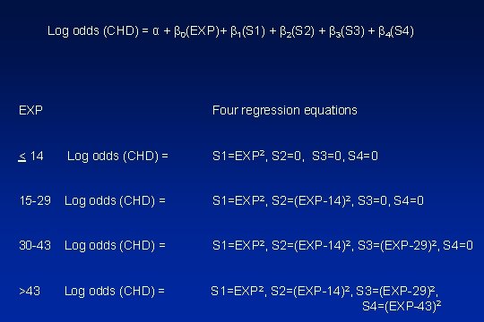
Log odds (CHD) = α + 0(EXP)+ 1(S 1) + 2(S 2) + 3(S 3) + 4(S 4) EXP Four regression equations < 14 Log odds (CHD) = S 1=EXP 2, S 2=0, S 3=0, S 4=0 15 -29 Log odds (CHD) = S 1=EXP 2, S 2=(EXP-14)2, S 3=0, S 4=0 30 -43 Log odds (CHD) = S 1=EXP 2, S 2=(EXP-14)2, S 3=(EXP-29)2, S 4=0 >43 Log odds (CHD) = S 1=EXP 2, S 2=(EXP-14)2, S 3=(EXP-29)2, S 4=(EXP-43)2

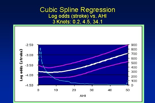
Cubic Spline Regression Log odds (stroke) vs. AHI 3 Knots: 0. 2, 4. 5, 34. 1

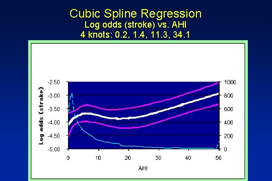
Cubic Spline Regression Log odds (stroke) vs. AHI 4 knots: 0. 2, 1. 4, 11. 3, 34. 1

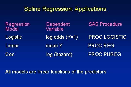
Spline Regression: Applications Regression Model Dependent Variable SAS Procedure Logistic log odds (Y=1) PROC LOGISTIC Linear mean Y PROC REG Cox log (hazard) PROC PHREG All models are linear functions of the predictors

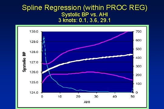
Spline Regression (within PROC REG) Systolic BP vs. AHI 3 knots: 0. 1, 3. 6, 29. 1

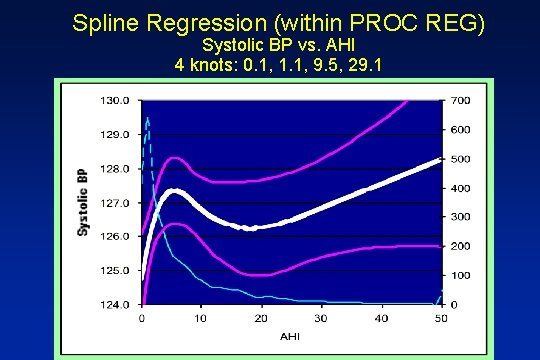
Spline Regression (within PROC REG) Systolic BP vs. AHI 4 knots: 0. 1, 1. 1, 9. 5, 29. 1

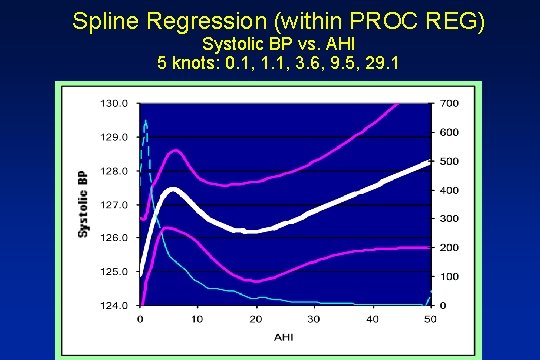
Spline Regression (within PROC REG) Systolic BP vs. AHI 5 knots: 0. 1, 1. 1, 3. 6, 9. 5, 29. 1

Spline Regression Key Advantages · Less restrictive assumptions · More regional flexibility · Does not rely on statistical hypothesis testing · Not as sensitive to the choice of cutoff points · Visual inspection of the dose-response pattern · Might be used to guide the choice of categories for traditional categorical analysis

Spline Regression Key Issues · Moderately sensitive to the number of knots (especially if only 3 are specified) · What do the “bumps and valleys” really mean? · Visual (subjective) interpretation - Consider the scale of the Y-axis - Consider the amount of data at the tail(s) - Straight line at the outermost segments