Exploring North Atlantic and North Pacific Decadal Climate

Exploring North Atlantic and North Pacific Decadal Climate Prediction Using Self. Organizing Maps Qinxue (Sharon) Gu 1 and Melissa Gervais* 1, 2, 3 1 Department of Meteorology and Atmospheric Science , The Pennsylvania State University, University Park, Pennsylvania 2 The Institute for Computational and Data Sciences, The Pennsylvania State University, University Park, Pennsylvania 3 Lamont-Doherty Earth Observatory, Columbia University, New York 1

Motivation Decadal climate prediction assesses the regional climate conditions and changes on a time scale of 10 to 30 years. It can provide important information to improve the decisions and policies. Decadal variability is impacted by natural external forcing, anthropogenic external forcing, and internal climate variability. Predicting internal variability remains a barrier to producing decadal climate predictions. This study explores the potential use of the self-organizing map (SOM) to: 1. Identify the internal climate variability 2. Measure theoretical decadal predictability of internal climate variability 3. Conduct decadal prediction within a long control simulation. 2

Data Community Earth System Model (CESM) 1 · Fully coupled version · Pre-industrial (1850) radiative forcing conditions December, January, and February (DJF) Sea Surface Temperature (SST) · 11 -year moving average Data Length: ~1500 years Resolution: ~1 degree Kay et al. 2015 3

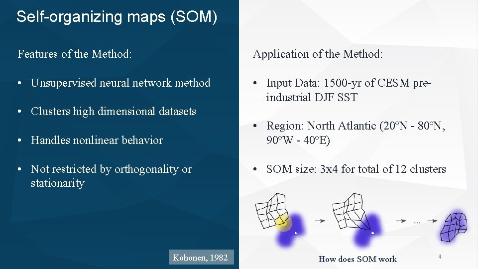
Self-organizing maps (SOM) Features of the Method: Application of the Method: • Unsupervised neural network method • Input Data: 1500 -yr of CESM preindustrial DJF SST • Clusters high dimensional datasets • Region: North Atlantic (20ºN - 80ºN, 90ºW - 40ºE) • Handles nonlinear behavior • Not restricted by orthogonality or stationarity Kohonen, 1982 • SOM size: 3 x 4 for total of 12 clusters How does SOM work 4

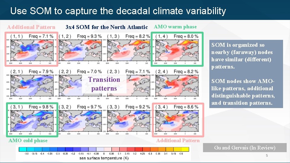
Use SOM to capture the decadal climate variability Additional Pattern 3 x 4 SOM for the North Atlantic AMO warm phase SOM is organized so nearby (faraway) nodes have similar (different) patterns. Transition patterns AMO cold phase SOM nodes show AMOlike patterns, additional distinguishable patterns, and transition patterns. Additional Pattern Gu and Gervais (In Review) 5

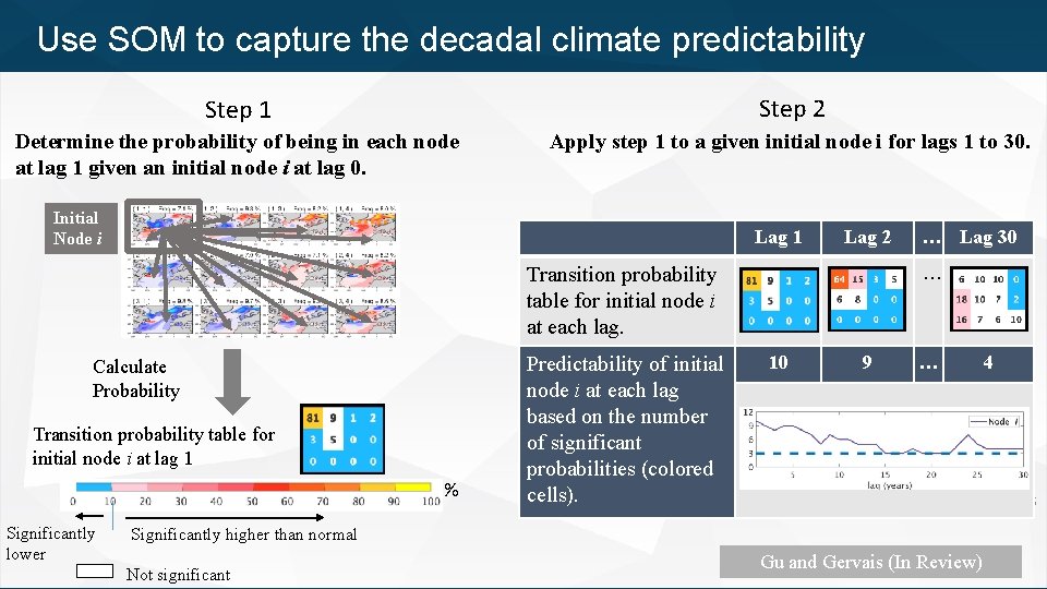
Use SOM to capture the decadal climate predictability Step 1 Step 2 Determine the probability of being in each node at lag 1 given an initial node i at lag 0. Apply step 1 to a given initial node i for lags 1 to 30. …… Initial Node i Lag 1 Lag 2 … Transition probability table for initial node i at each lag. Calculate Probability Transition probability table for initial node i at lag 1 % Significantly lower Predictability of initial node i at each lag based on the number of significant probabilities (colored cells). … Lag 30 10 9 … 6 Significantly higher than normal Not significant 4 Gu and Gervais (In Review)

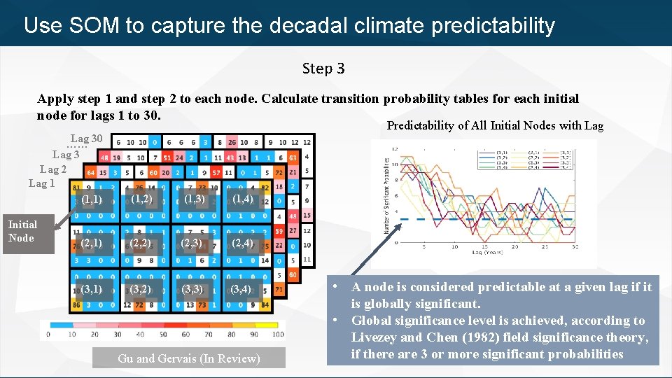
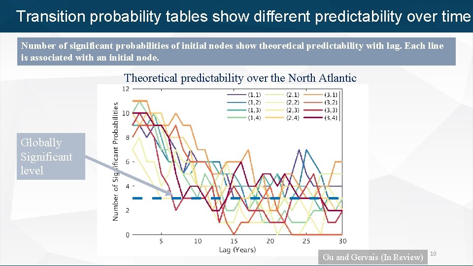
Use SOM to capture the decadal climate predictability Step 3 Apply step 1 and step 2 to each node. Calculate transition probability tables for each initial node for lags 1 to 30. Lag 30 …… Lag 3 Lag 2 Lag 1 (1, 1) Initial Node Predictability of All Initial Nodes with Lag (1, 2) (1, 3) (1, 4) (2, 1) (2, 2) (2, 3) (2, 4) (3, 1) (3, 2) (3, 3) (3, 4) Gu and Gervais (In Review) • A node is considered predictable at a given lag if it is globally significant. • Global significance level is achieved, according to Livezey and Chen (1982) field significance theory, if there are 3 or more significant probabilities

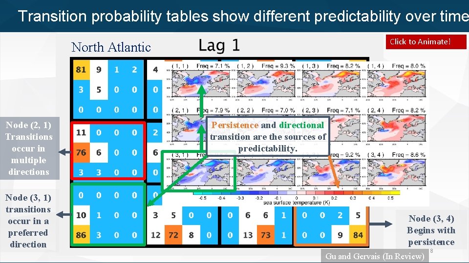
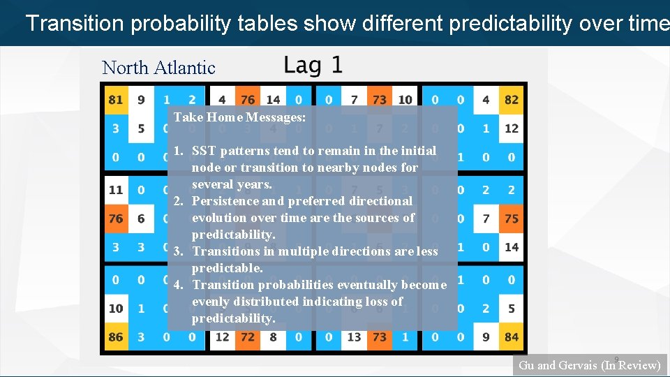
Transition probability tables show different predictability over time Click to Animate! North Atlantic Node (2, 1) Transitions occur in multiple directions Node (3, 1) transitions occur in a preferred direction Persistence and directional transition are the sources of predictability. Node (3, 4) Begins with persistence Gu and Gervais (In Review) 8

Transition probability tables show different predictability over time North Atlantic Take Home Messages: 1. SST patterns tend to remain in the initial node or transition to nearby nodes for several years. 2. Persistence and preferred directional evolution over time are the sources of predictability. 3. Transitions in multiple directions are less predictable. 4. Transition probabilities eventually become evenly distributed indicating loss of predictability. 9 Gu and Gervais (In Review)

Transition probability tables show different predictability over time Number of significant probabilities of initial nodes show theoretical predictability with lag. Each line is associated with an initial node. Theoretical predictability over the North Atlantic Globally Significant level Gu and Gervais (In Review) 10

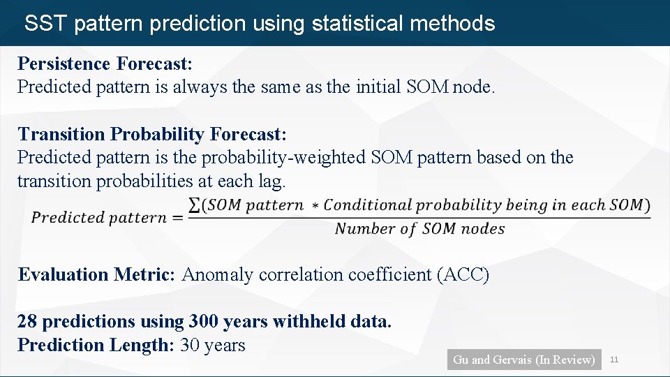
SST pattern prediction using statistical methods Persistence Forecast: Predicted pattern is always the same as the initial SOM node. Transition Probability Forecast: Predicted pattern is the probability-weighted SOM pattern based on the transition probabilities at each lag. Evaluation Metric: Anomaly correlation coefficient (ACC) 28 predictions using 300 years withheld data. Prediction Length: 30 years Gu and Gervais (In Review) 11

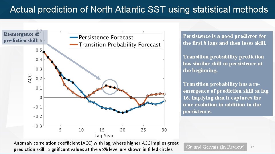
Actual prediction of North Atlantic SST using statistical methods Reemergence of prediction skill Persistence is a good predictor for the first 8 lags and then loses skill. Transition probability prediction has similar skill to persistence at the beginning. Transition probability has a reemergence of prediction skill at lag 16, implying that it captures the true evolution in addition to the persistence. Anomaly correlation coefficient (ACC) with lag, where higher ACC implies great prediction skill. Significant values at the 95% level are shown in filled circles. Gu and Gervais (In Review) 12

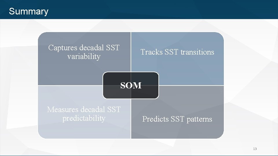
Summary Captures decadal SST variability Tracks SST transitions SOM Measures decadal SST predictability Predicts SST patterns 13

References Gu, Q. & Gervais, M. Exploring north atlantic and north pacific decadal climate prediction using self-organizing maps (In Review) Kay, J. E. , Deser, C. , Phillips, A. , Mai, A. , Hannay, C. , Strand, G. , et al. (2014). The Community Earth System Model (CESM) Large Ensemble Project: A Community Resource for Studying Climate Change in the Presence of Internal Climate Variability. Bulletin of the American Meteorological Society, 96(8), 1333– 1349. https: //doi. org/10. 1175/BAMS-D-13 -00255. 1 Kohonen, T. (1982). Self-organized formation of topologically correct feature maps. Biological Cybernetics. https: //doi. org/10. 1007/BF 00337288 Kosaka, Y. , & Xie, S. P. (2013). Recent global-warming hiatus tied to equatorial Pacific surface cooling. Nature, 501(7467), 403– 407. https: //doi. org/10. 1038/nature 12534 Livezey, R. E. , & Chen, W. Y. (1983). Statistical field significance and its determination by Monte Carlo techniques. Monthly Weather Review, 111(1), 46– 59. https: //doi. org/10. 1175/1520 -0493(1983)111<0046: SFSAID>2. 0. CO; 2 Newman, M. , Alexander, M. A. , Ault, T. R. , Cobb, K. M. , Deser, C. , Di Lorenzo, E. , et al. (2016). The Pacific decadal oscillation, revisited. Journal of Climate, 29(12), 4399– 4427. https: //doi. org/10. 1175/JCLI-D-15 -0508. 1 Thank you for watching! If you have any thoughts/comments/suggestions, please contact with us. Qinxue (Sharon) Gu: qzg 18@psu. edu 14 Melissa Gervais: mmg 62@psu. edu