Exploring Large Graphs in 3 D Hyperpbolic Space

Exploring Large Graphs in 3 D Hyperpbolic Space And Graph. Splatting: Visualizing Graphs as Continuous Fields

Exploring Large Graphs in 3 D Hyperbolic Space (1998) Tamera Munzner Stanford University

Exploring Large Graphs in 3 D Hyperbolic Space (1998) § Software system that handles much larger graphs and supports dynamic exploration (Called H 3) § Developed algorithms for graph layout and drawing § Drawn in 3 D hyperbolic space to show a large neighborhood around a node of interest

Spanning Trees § Need to find a spanning tree to compute layout. Spanning tree influences the system’s visual impact § Can use BFS spanning tree, but exploiting domain-specific knowledge creates better mental model § This means, for each node, deciding some parent child relationship with the edges.

Sample domain specific spanning trees § Web Site- URL encodes the site’s directory structure. § Function call graph- Compiler analysis and runtime profiling must be done to find where procedure is being called most of the time. The resulting H 3 layout makes it easier for software engineers to understand

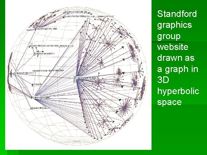
Standford graphics group website drawn as a graph in 3 D hyperbolic space

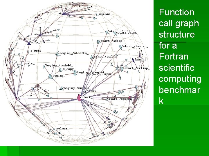
Function call graph structure for a Fortran scientific computing benchmar k

Layout § Basis is cone tree method § Instead of laying nodes on linear circumference of a cone’s mouth, H 3 lays nodes out on a surface of a hemisphere § The cone widens to its maximum extent § Cone body flattens out into a disk at base of hemisphere

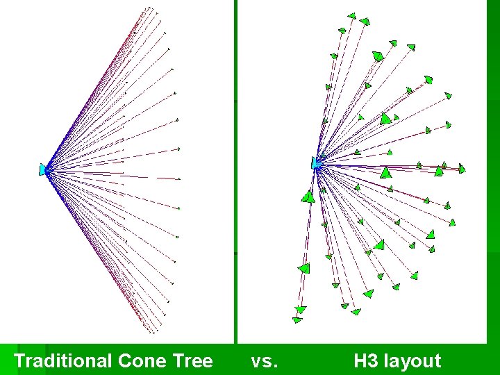
Traditional Cone Tree vs. H 3 layout

Layout Algorithm § It requires 2 passes § A bottom-up pass to estimate the radius needed for each hemisphere to accommodate all its children § A top-down pass to place each child node on its parental hemisphere's surface.

Layout (cont) § Circle packing problem- child hemispheres on the surface of their parent § Solution- lay out children in concetric bands around the hemisphere’s pole. The amount of room each node needs is directly proportional to the total number of its descendants.

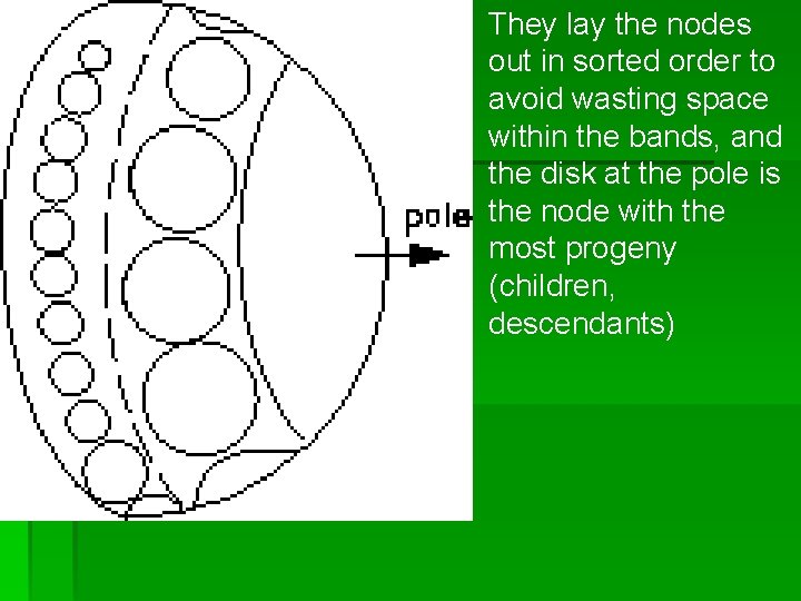
They lay the nodes out in sorted order to avoid wasting space within the bands, and the disk at the pole is the node with the most progeny (children, descendants)

Hemispherical Layout § Area of hemisphere, 2πr, increases polynomially with respect to its radius in Euclidean space § Area of hemisphere, 2πsinh 2(r), increases exponentially § In hyperbolic geometry, you can map the entire infinite space into a finite portion of Euclidean space § Is effective because the tree is laid out in a mathematical space having a exponential “amount of room” in direction of the hemisphere’s growth § They chose the Klein hyperbolic geometry model because motions can be expressed as 4 x 4 matrices.

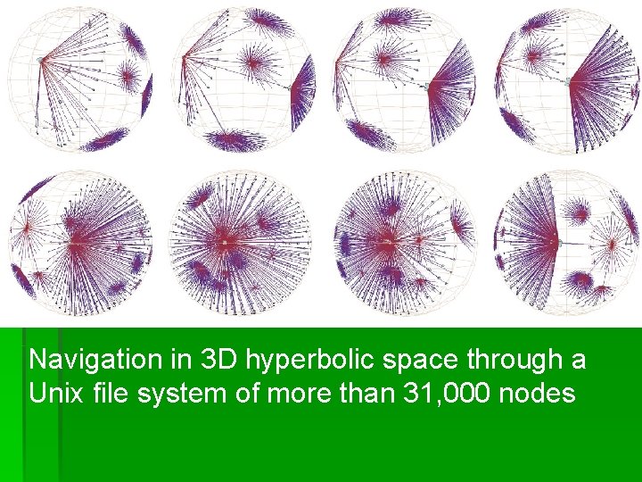
Navigation in 3 D hyperbolic space through a Unix file system of more than 31, 000 nodes

Drawing § Only a local neighborhood of nodes in the graph will be visible at any given time. This is because the projection from hyperbolic to Euclidean space guarantees that nodes sufficiently far from the center will project to less than a single pixel.

Drawing (cont) § Designed adaptive drawing algorithm to always maintain a target frame rate § A high constant framerate results from drawing only as much of the neighborhood around a center point as much as allotted time permits § When user is idle, the system fills in more of the surrounding scene.

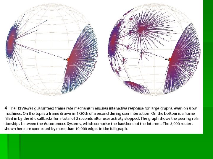
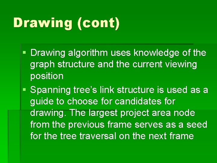
Drawing (cont) § Drawing algorithm uses knowledge of the graph structure and the current viewing position § Spanning tree’s link structure is used as a guide to choose for candidates for drawing. The largest project area node from the previous frame serves as a seed for the tree traversal on the next frame

Scaffolding for attributes § Can show dynamic or static attributes. § By color and line-width coding, text labels, and filtering § Example: Can show paths taken by Web Users by highlight those nodes or coloring the edges § Color of edge can represent if inward edge or outward edge

Local Orientation § When user clicks on node, it is highlighted and undergoes an animated transition to the center of the sphere. This minimizes occlusion of nodes and labels § Ancestors appear on left and descendents appear on right

Local Orientation (cont) § It draws links to and out of node even if doesn’t draw node at other end. § This presence of undetermined link during motion hints user of something interesting in that direction

Context of part in whole § Hyperbolic space very effectively presents a large area around a focus node § User can see enough of the distant subtrees to identify dense and sparse ones

Graph as index § Integrate H 3 Viewer with other graph views like 2 D file viewer § Graph structure becomes one way to index the information. This becomes useful for finding patterns in a different type of view

Conclusion § It can handle graphs that are very large(more than 100, 000 edges) § Manipulates by using backbone spanning tree § 3 D hyperbolic space allows large amount of context around a focus point § Layout is good balance of information density and clutter § Maintains guaranteed frame rate § I downloaded movies of it and demo program from website

Graph. Splatting: Visualizing Graphs as Continuous Fields (2003) Robert van Liere and Wim de Leeuw

Graph. Splatting: Visualizing Graphs as Continous Fields § Transforms a graph into a 2 D scalar field § Scalar field can be rendered as a color-coded map, a height field, or a set of contours § Allows visualization of large graphs without cluttering (overview of graph) § It provides density information of the graph (assuming that graph Layout algorithm uses density of vertices as a characteristic) That is, How vertices placed relative to each other means something

Related Work § This work was inspired by Theme. Scape, a technique which conveys information about topics in text documents. They are 3 D landscapes of information that are constructed from documents to show strength of themes in a document

Graph. Slatting technique § Central assumption is that the density of vertices is an important characteristic of layout used by a graph § Some layouts that use this are the spring mass technique and edge length minimization technique

Splatting § Projects each vertex of the graph onto 2 D scalar field using splatting function. § Instead of showing individual vertices, continuous variation in density is shown § Each vertex contributes to the field with a 2 D Gaussian shaped basis function. Field is obtained by adding all the contributions. -> splat field

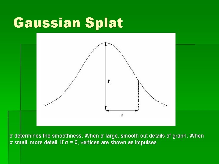
Gaussian Splat σ determines the smoothness. When σ large, smooth out details of graph. When σ small, more detail. If σ = 0, vertices are shown as impulses

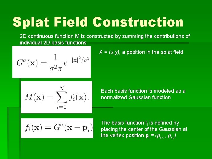
Splat Field Construction 2 D continuous function M is constructed by summing the contributions of individual 2 D basis functions X = (x, y), a position in the splat field Each basis function is modeled as a normalized Gaussian function The basis function fi is defined by placing the center of the Gaussian at the vertex position pi = (pi, x , pi, y)

Splat field construction (cont) § Splat field is done on a grid with user controlled resolution § Gaussian functions are discretized and added to the cells grid § Contribution to each splat to a pixel in the grid is estimated by using the distance between the vertex position and the center of the pixel

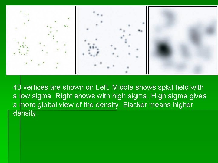
40 vertices are shown on Left. Middle shows splat field with a low sigma. Right shows with high sigma. High sigma gives a more global view of the density. Blacker means higher density.

Splat Field Visualization § Important to realize that underlying data is a graph. Splat field is often combined with discrete representations that can be rendered on top of the splat field. § Color coding. 2 D view of the field which the value is shown using color. § Height map § Isovalue contours. Can be used to show the boundary of specific clusters

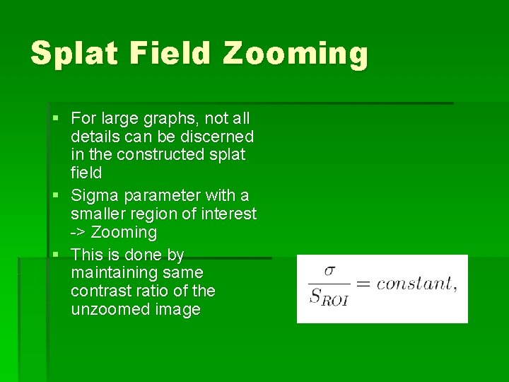
Splat Field Zooming § For large graphs, not all details can be discerned in the constructed splat field § Sigma parameter with a smaller region of interest -> Zooming § This is done by maintaining same contrast ratio of the unzoomed image

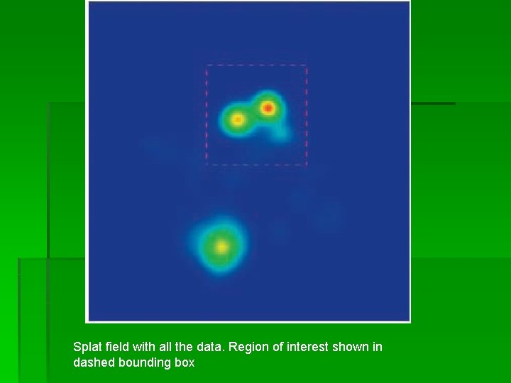
Splat field with all the data. Region of interest shown in dashed bounding box

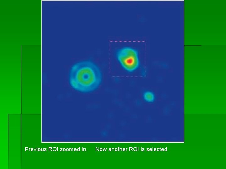
Previous ROI zoomed in. Now another ROI is selected

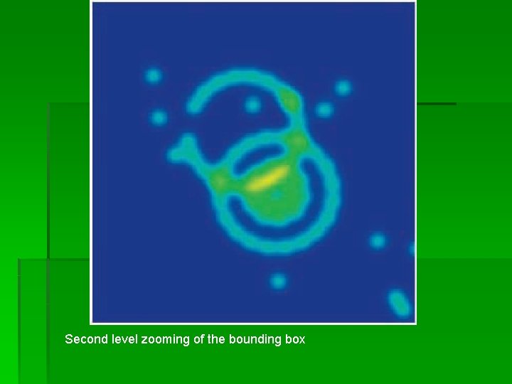
Second level zooming of the bounding box

Combining Splat Fields with Texture Fields § Gaussian function is limited in the frequency domain § The sum of Gaussian functions will have the same spectral properties as a single Gaussian function. So spectrum of splat field is restricted to lower frequencies § This property is used to map an additional scalar field. Remaining higher frequencies are used for a texture that represents additional scalar data

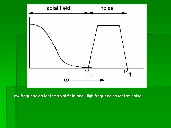
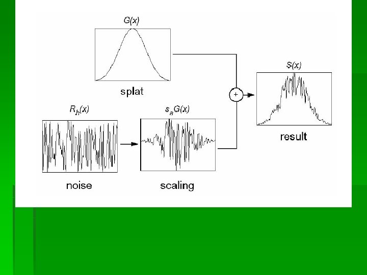
Low frequencies for the splat field and High frequencies for the noise

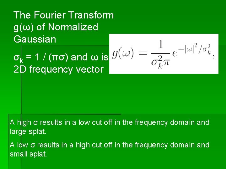
The Fourier Transform g(ω) of Normalized Gaussian σk = 1 / (πσ) and ω is 2 D frequency vector A high σ results in a low cut off in the frequency domain and large splat. A low σ results in a high cut off in the frequency domain and small splat.

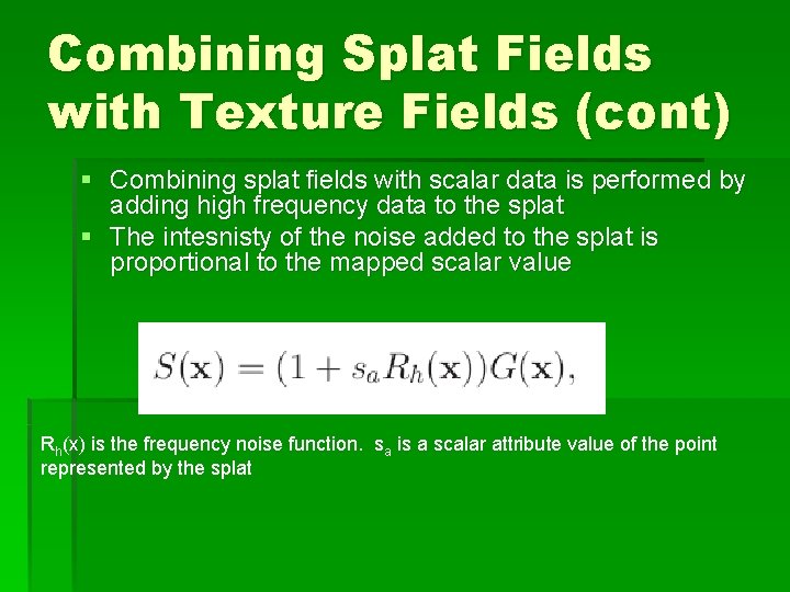
Combining Splat Fields with Texture Fields (cont) § Combining splat fields with scalar data is performed by adding high frequency data to the splat § The intesnisty of the noise added to the splat is proportional to the mapped scalar value Rh(x) is the frequency noise function. sa is a scalar attribute value of the point represented by the splat

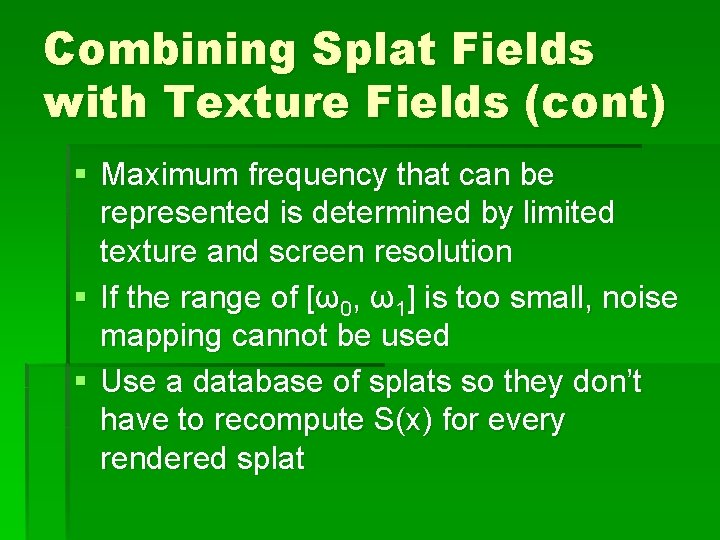
Combining Splat Fields with Texture Fields (cont) § Maximum frequency that can be represented is determined by limited texture and screen resolution § If the range of [ω0, ω1] is too small, noise mapping cannot be used § Use a database of splats so they don’t have to recompute S(x) for every rendered splat

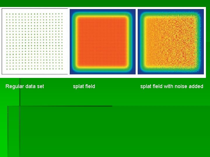
Regular data set splat field with noise added

Hardware Implementation § Gaussian Function represented as textured polygon, rendered to offscreen buffer with additive blending enabled § Optimal rendering, max splat value would map to max pixel value § Due to limited dept of frame buffer, and to additive blending of unknown number of splats, the maximum intensity of splat field is unknown

Hardware Implementation (cont) § Use adaptive algorithm to get optimal intensity mapping § Optimal intensity is a value at least 80% of max intensity of frame buffer § Algorithm scales intensity of all splats such that max intensity of splat field is close to max intensity of frame buffer

Hardware Implementation (cont) § Algorithm implemented by first rendering splat field with estimated splat intensity scaling. Imax of splat field is scanned for. § 3 cases for Imax

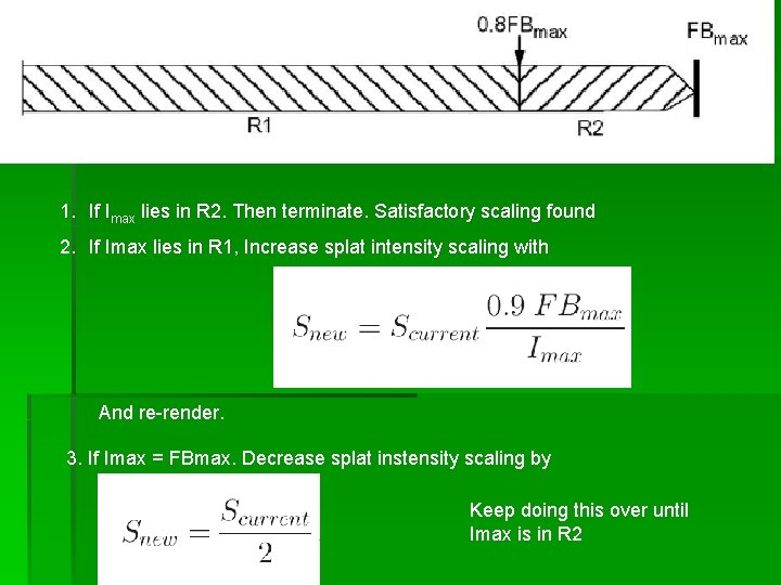
1. If Imax lies in R 2. Then terminate. Satisfactory scaling found 2. If Imax lies in R 1, Increase splat intensity scaling with And re-render. 3. If Imax = FBmax. Decrease splat instensity scaling by Keep doing this over until Imax is in R 2

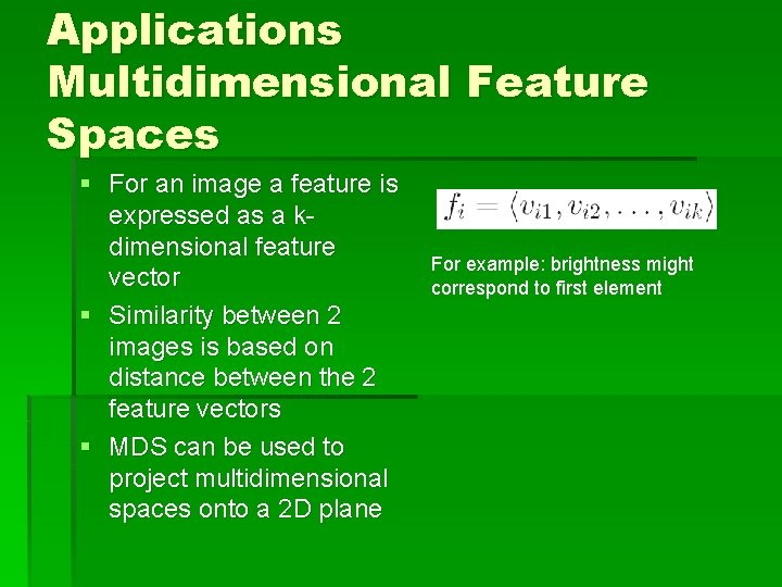
Applications Multidimensional Feature Spaces § For an image a feature is expressed as a kdimensional feature vector § Similarity between 2 images is based on distance between the 2 feature vectors § MDS can be used to project multidimensional spaces onto a 2 D plane For example: brightness might correspond to first element

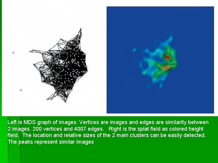
Left is MDS graph of images. Vertices are images and edges are similarity between 2 images. 200 vertices and 4007 edges. Right is the splat field as colored height field. The location and relative sizes of the 2 main clusters can be easily detected. The peaks represent similar images

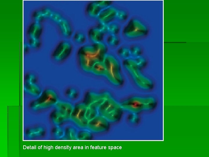
Detail of high density area in feature space

Application IEEE Vis Citation Index § Input data are Bib. Te. X entries of papers in the IEEE Vis’XX conferences and all references between papers in the set § 672 Bib. Te. X entries, 1044 references § Also name session where paper was collected

Application IEEE Vis Citation Index (cont) § Graph was made where vertices = papers and edges = references § Used spring mass graph layout § Referencing papers are attracted to each other § Goal: test hypothesis: topics in visualization could be identified by using reference information

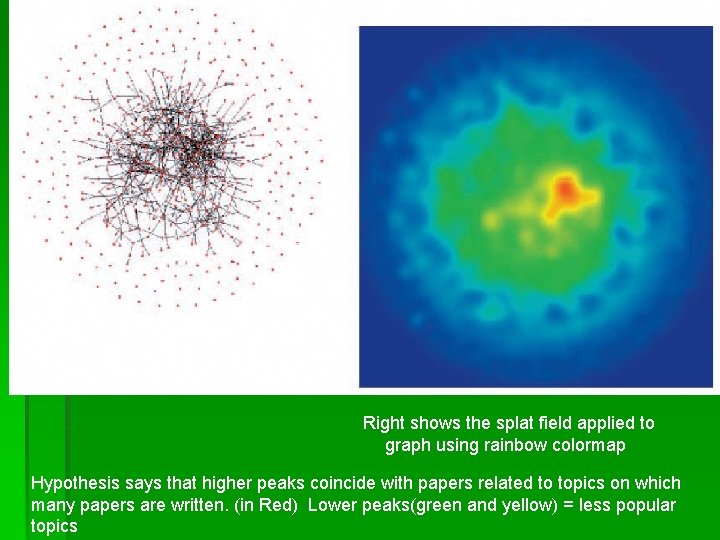
Right shows the splat field applied to graph using rainbow colormap Hypothesis says that higher peaks coincide with papers related to topics on which many papers are written. (in Red) Lower peaks(green and yellow) = less popular topics

Application IEEE Vis Citation Index (cont) § To validate hypothesis, used session names to show what topic paper belongs to § Noise mapping used to combine splatmap with info about the session name of paper § Occurrence of “flow” or “volume” in session name linked to Boolean attribute to noise mapping § Papers menitioned in sessions are rendered as noisy splats

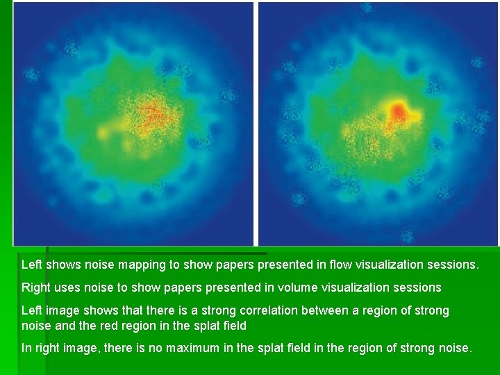
Left shows noise mapping to show papers presented in flow visualization sessions. Right uses noise to show papers presented in volume visualization sessions Left image shows that there is a strong correlation between a region of strong noise and the red region in the splat field In right image, there is no maximum in the splat field in the region of strong noise.

Application IEEE Vis Citation Index (cont) § Since noise regions are disjoint, the assumption that visualization topics can be identified is valid § For flow viz, strong correlation between the noise field and splat field. Not so for vol viz. § Noise fields show small regions out of “primary region” of splat field. This is because these papers do not reference other papers. § Flow papers tend to reference other papers and Volume papers do not.

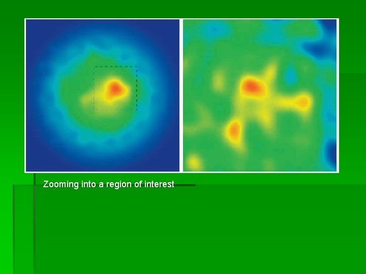
Zooming into a region of interest

Discussion/Conclusion § Overview of arbitrarily large graphs can be produced § Visualization of splat fields presents density information. Graph layout must have meaning between vertices spaces § Noise mapping can be used to present secondary scalar field.