Exploring Intrinsic Structures from Samples Supervised Unsupervised and

Exploring Intrinsic Structures from Samples: Supervised, Unsupervised, and Semisupervised Frameworks Supervised by Prof. Xiaoou Tang & Prof. Jianzhuang Liu

Outline • Notations & introductions • Trace Ratio Optimization Preserve sample feature structures Dimensionality reduction Tensor Subspace Learning Explore the geometric structures and feature domain relations concurrently • Correspondence Propagation Outline

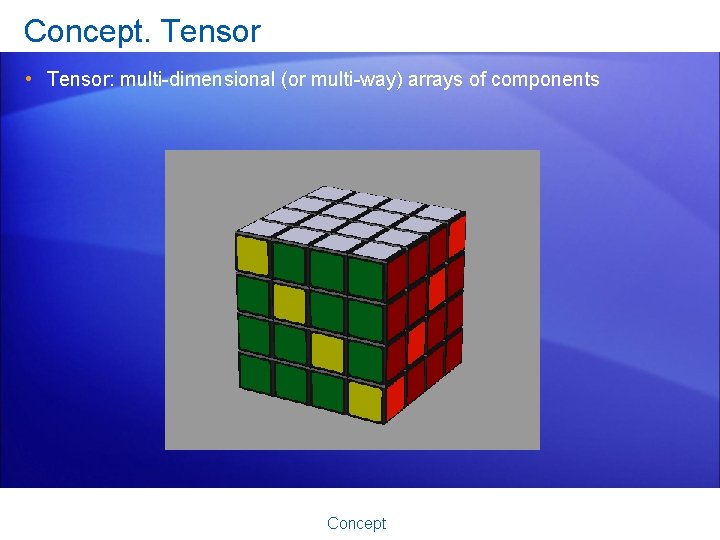
Concept. Tensor • Tensor: multi-dimensional (or multi-way) arrays of components Concept

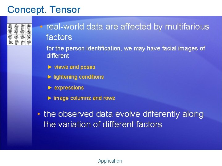
Concept. Tensor • real-world data are affected by multifarious factors for the person identification, we may have facial images of different ► views and poses ► lightening conditions ► expressions ► image columns and rows • the observed data evolve differently along the variation of different factors Application

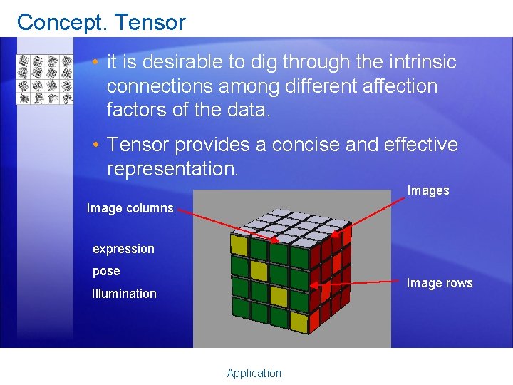
Concept. Tensor • it is desirable to dig through the intrinsic connections among different affection factors of the data. • Tensor provides a concise and effective representation. Images Image columns expression pose Image rows Illumination Application

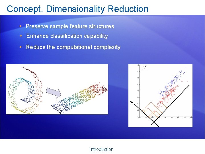
Concept. Dimensionality Reduction • Preserve sample feature structures • Enhance classification capability • Reduce the computational complexity Introduction

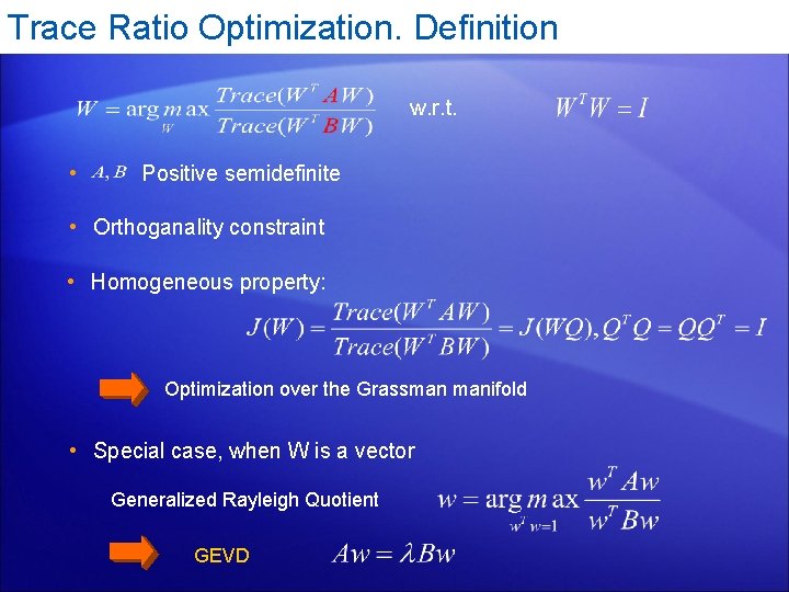
Trace Ratio Optimization. Definition w. r. t. • Positive semidefinite • Orthoganality constraint • Homogeneous property: Optimization over the Grassman manifold • Special case, when W is a vector Generalized Rayleigh Quotient GEVD

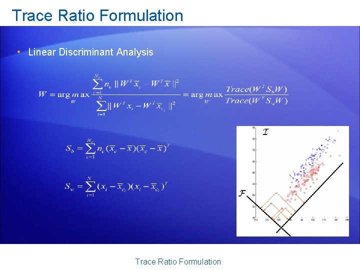
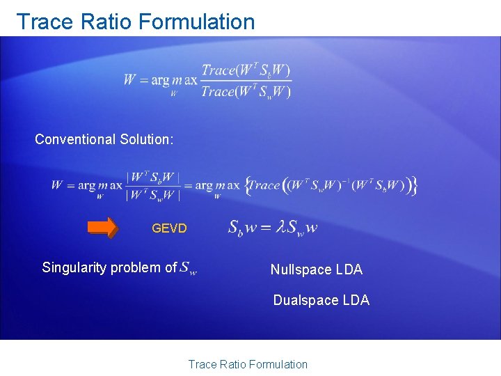
Trace Ratio Formulation • Linear Discriminant Analysis Trace Ratio Formulation

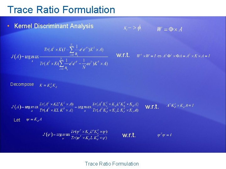
Trace Ratio Formulation • Kernel Discriminant Analysis w. r. t. Decompose w. r. t. Let w. r. t. Trace Ratio Formulation

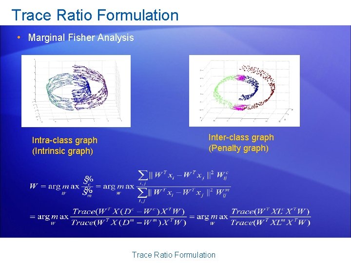
Trace Ratio Formulation • Marginal Fisher Analysis Intra-class graph (Intrinsic graph) Inter-class graph (Penalty graph) Trace Ratio Formulation

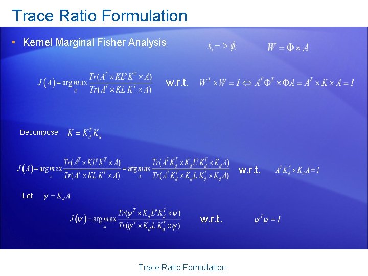
Trace Ratio Formulation • Kernel Marginal Fisher Analysis w. r. t. Decompose w. r. t. Let w. r. t. Trace Ratio Formulation

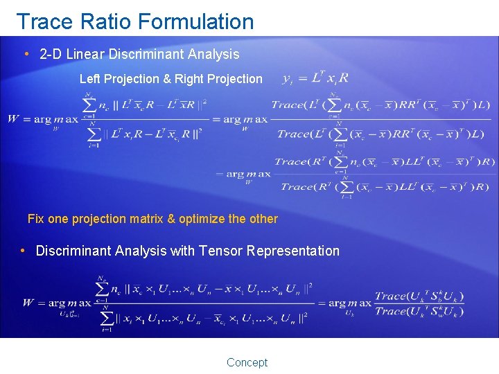
Trace Ratio Formulation • 2 -D Linear Discriminant Analysis Left Projection & Right Projection Fix one projection matrix & optimize the other • Discriminant Analysis with Tensor Representation Concept

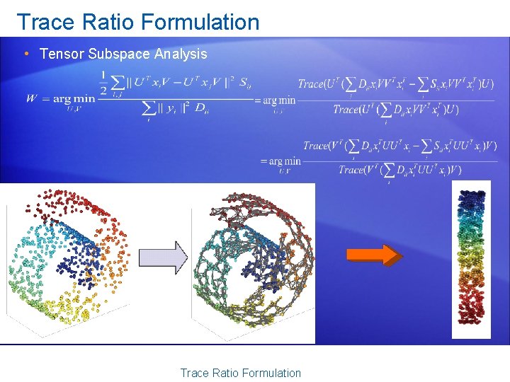
Trace Ratio Formulation • Tensor Subspace Analysis Trace Ratio Formulation

Trace Ratio Formulation Conventional Solution: GEVD Singularity problem of Nullspace LDA Dualspace LDA Trace Ratio Formulation

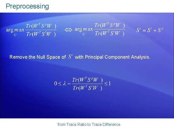
Preprocessing Remove the Null Space of with Principal Component Analysis. from Trace Ratio to Trace Difference

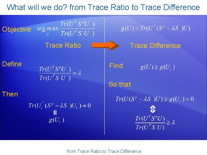
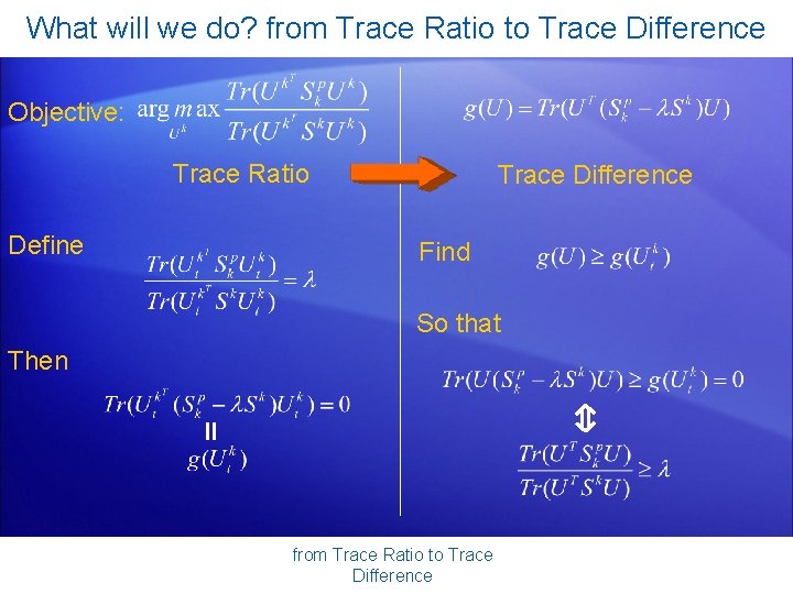
What will we do? from Trace Ratio to Trace Difference Objective: Trace Ratio Define Trace Difference Find So that Then from Trace Ratio to Trace Difference

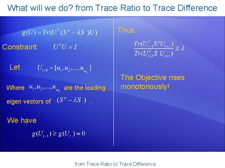
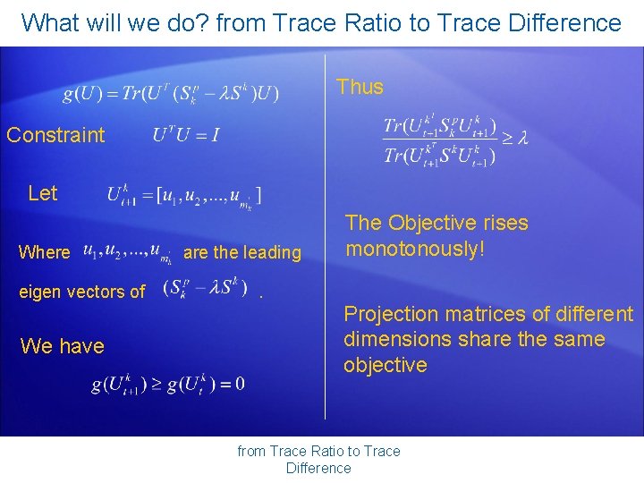
What will we do? from Trace Ratio to Trace Difference Thus Constraint Let Where eigen vectors of are the leading The Objective rises monotonously! . We have from Trace Ratio to Trace Difference

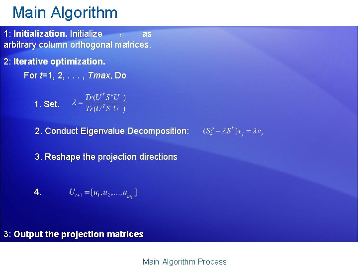
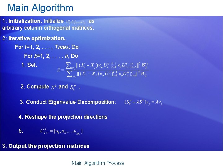
Main Algorithm 1: Initialization. Initialize as arbitrary column orthogonal matrices. 2: Iterative optimization. For t=1, 2, . . . , Tmax, Do 1. Set. 2. Conduct Eigenvalue Decomposition: 3. Reshape the projection directions 4. 3: Output the projection matrices Main Algorithm Process

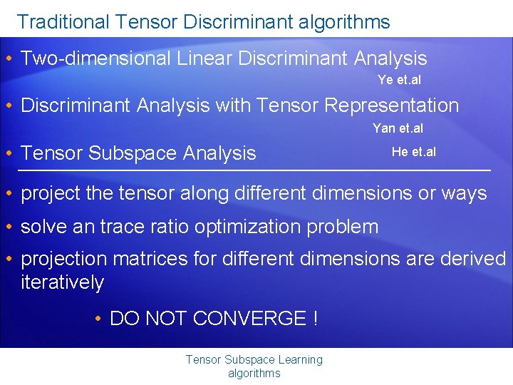
Traditional Tensor Discriminant algorithms • Two-dimensional Linear Discriminant Analysis Ye et. al • Discriminant Analysis with Tensor Representation Yan et. al • Tensor Subspace Analysis He et. al • project the tensor along different dimensions or ways • solve an trace ratio optimization problem • projection matrices for different dimensions are derived iteratively • DO NOT CONVERGE ! Tensor Subspace Learning algorithms

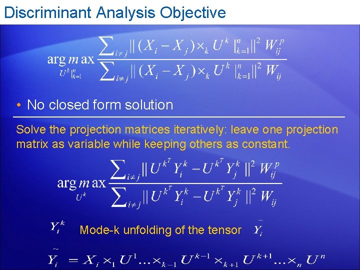
Discriminant Analysis Objective • No closed form solution Solve the projection matrices iteratively: leave one projection matrix as variable while keeping others as constant. Mode-k unfolding of the tensor

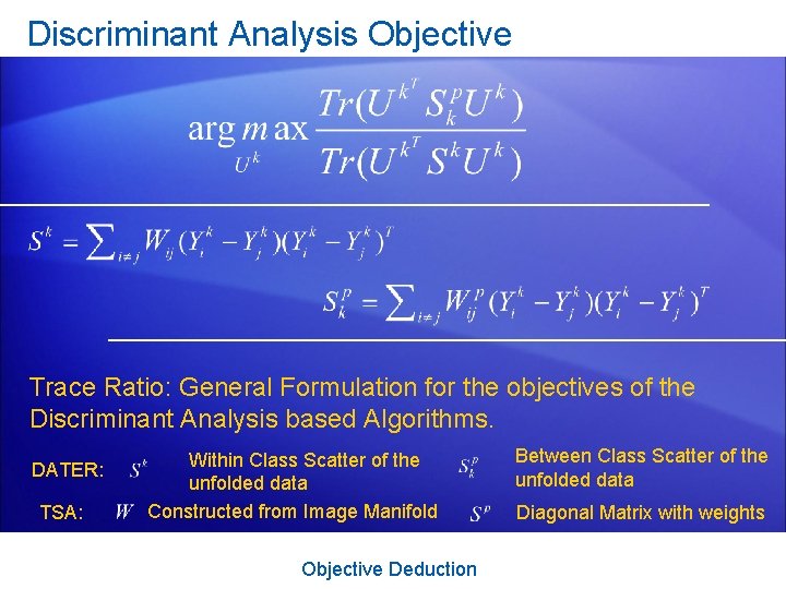
Discriminant Analysis Objective Trace Ratio: General Formulation for the objectives of the Discriminant Analysis based Algorithms. DATER: TSA: Within Class Scatter of the unfolded data Constructed from Image Manifold Objective Deduction Between Class Scatter of the unfolded data Diagonal Matrix with weights

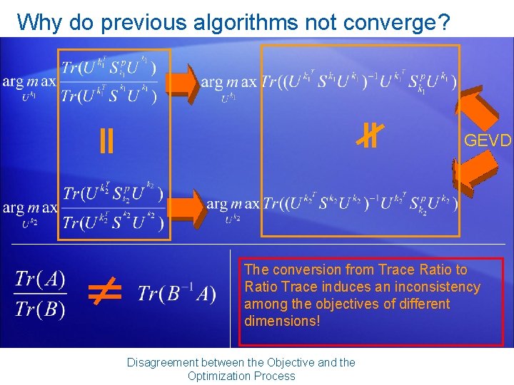
Why do previous algorithms not converge? GEVD The conversion from Trace Ratio to Ratio Trace induces an inconsistency among the objectives of different dimensions! Disagreement between the Objective and the Optimization Process

What will we do? from Trace Ratio to Trace Difference Objective: Trace Ratio Define Trace Difference Find So that Then from Trace Ratio to Trace Difference

What will we do? from Trace Ratio to Trace Difference Thus Constraint Let Where eigen vectors of We have are the leading The Objective rises monotonously! . Projection matrices of different dimensions share the same objective from Trace Ratio to Trace Difference

Main Algorithm 1: Initialization. Initialize as arbitrary column orthogonal matrices. 2: Iterative optimization. For t=1, 2, . . . , Tmax, Do For k=1, 2, . . . , n, Do 1. Set. 2. Compute and . 3. Conduct Eigenvalue Decomposition: 4. Reshape the projection directions 5. 3: Output the projection matrices Main Algorithm Process

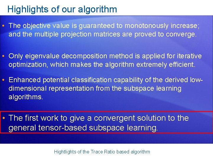
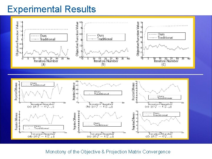
Highlights of our algorithm • The objective value is guaranteed to monotonously increase; and the multiple projection matrices are proved to converge. • Only eigenvalue decomposition method is applied for iterative optimization, which makes the algorithm extremely efficient. • Enhanced potential classification capability of the derived lowdimensional representation from the subspace learning algorithms. • The first work to give a convergent solution to the general tensor-based subspace learning. Hightlights of the Trace Ratio based algorithm

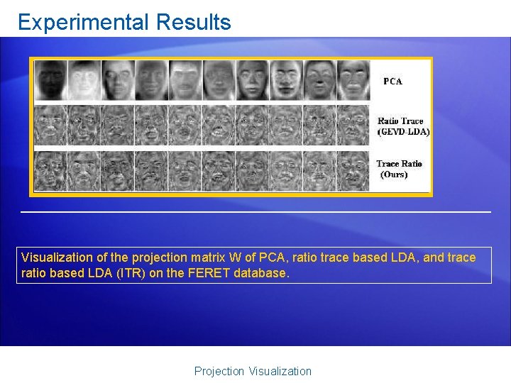
Experimental Results Visualization of the projection matrix W of PCA, ratio trace based LDA, and trace ratio based LDA (ITR) on the FERET database. Projection Visualization

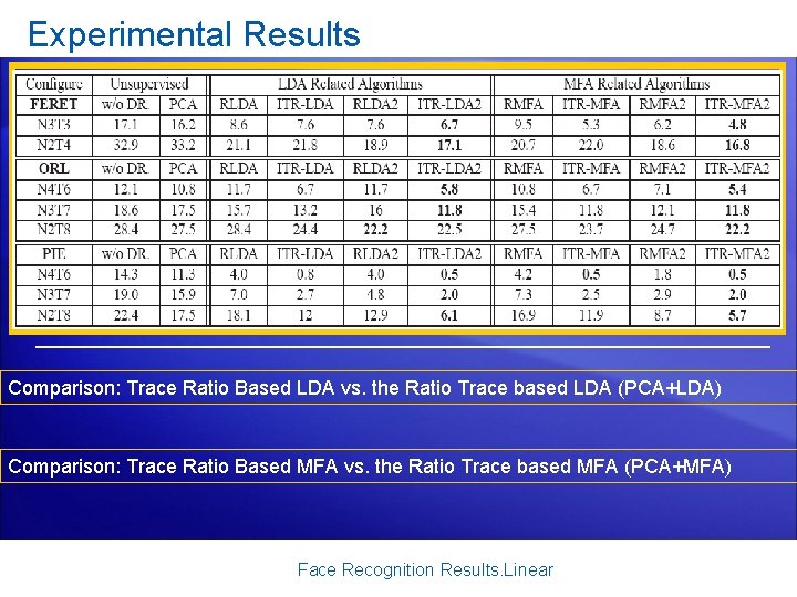
Experimental Results Comparison: Trace Ratio Based LDA vs. the Ratio Trace based LDA (PCA+LDA) Comparison: Trace Ratio Based MFA vs. the Ratio Trace based MFA (PCA+MFA) Face Recognition Results. Linear

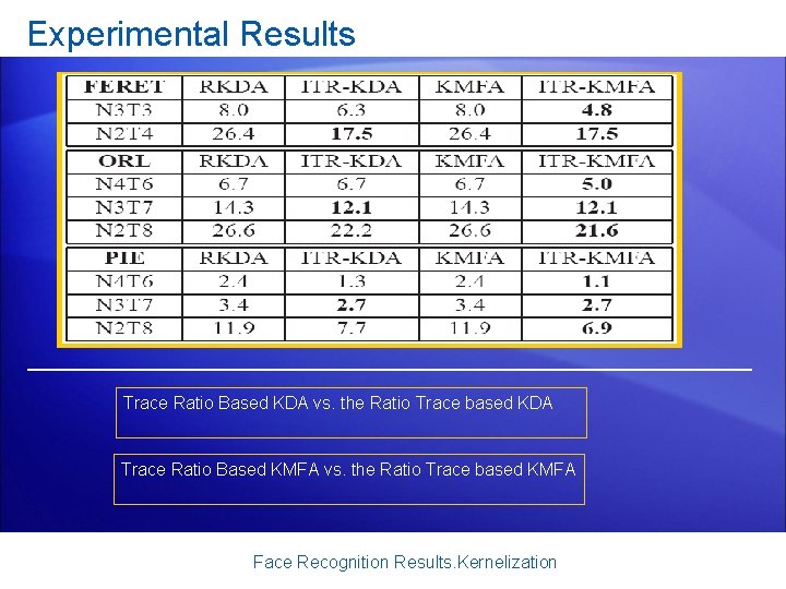
Experimental Results Trace Ratio Based KDA vs. the Ratio Trace based KDA Trace Ratio Based KMFA vs. the Ratio Trace based KMFA Face Recognition Results. Kernelization

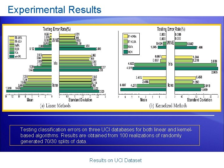
Experimental Results Testing classification errors on three UCI databases for both linear and kernelbased algorithms. Results are obtained from 100 realizations of randomly generated 70/30 splits of data. Results on UCI Dataset

Experimental Results Monotony of the Objective & Projection Matrix Convergence

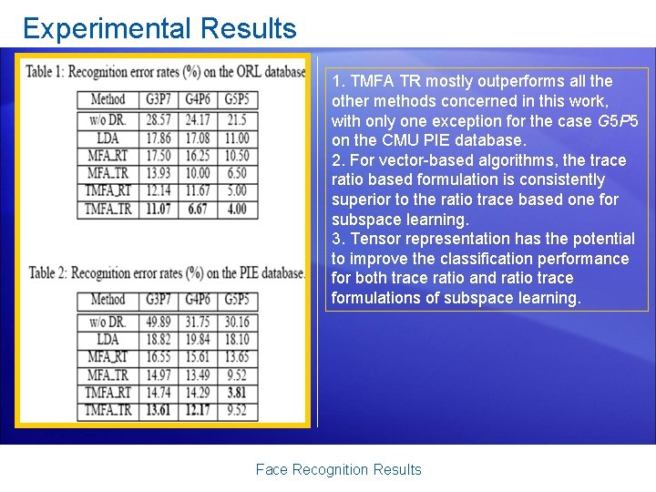
Experimental Results 1. TMFA TR mostly outperforms all the other methods concerned in this work, with only one exception for the case G 5 P 5 on the CMU PIE database. 2. For vector-based algorithms, the trace ratio based formulation is consistently superior to the ratio trace based one for subspace learning. 3. Tensor representation has the potential to improve the classification performance for both trace ratio and ratio trace formulations of subspace learning. Face Recognition Results

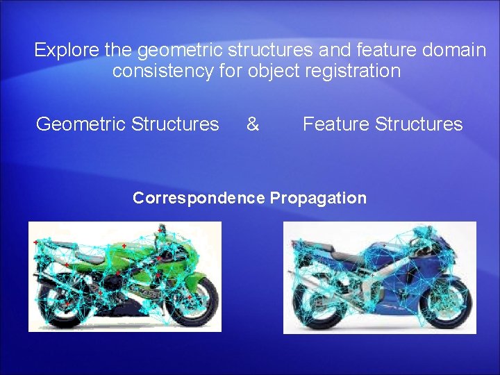
Explore the geometric structures and feature domain consistency for object registration Geometric Structures & Feature Structures Correspondence Propagation

Aim • Objects are represented as sets of feature points • Seek a mapping of features from sets of different cardinalities • Exploit the geometric structures of sample features • Introduce human interaction for correspondence guidance Objective

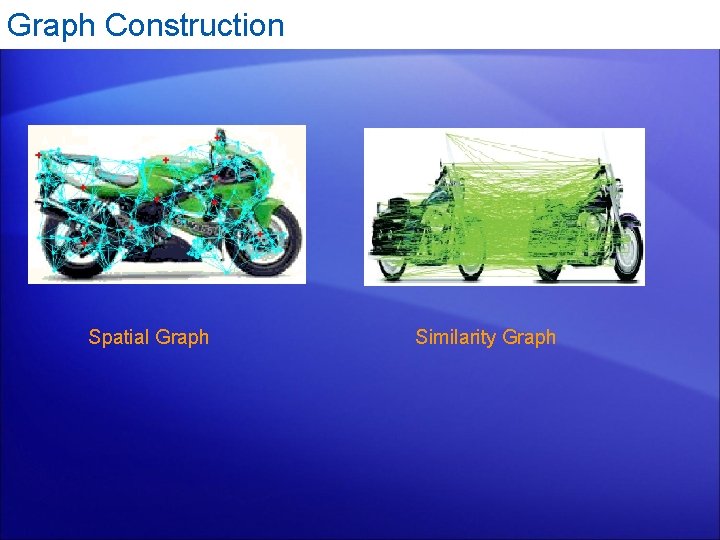
Graph Construction Spatial Graph Similarity Graph

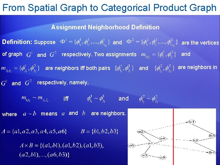
From Spatial Graph to Categorical Product Graph Assignment Neighborhood Definition: Suppose of graph and and respectively, namely, and iff where means and respectively. Two assignments are neighbors iff both pairs and are the vertices and are neighbors in

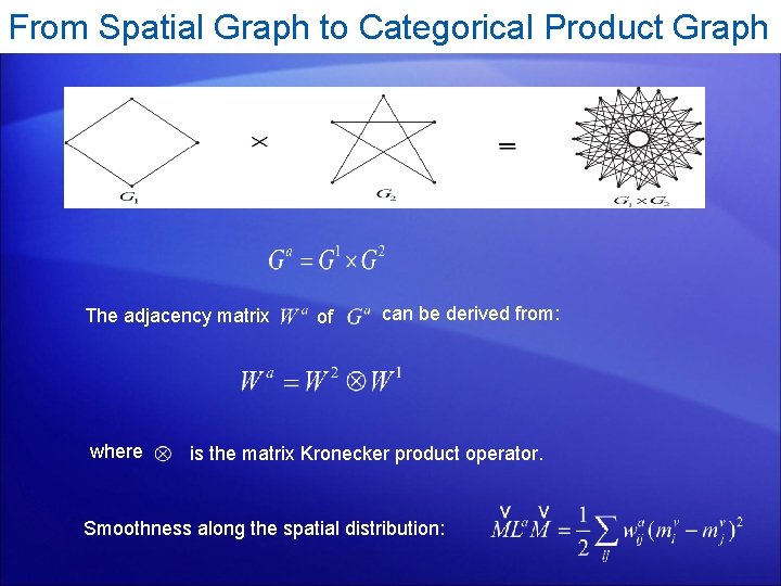
From Spatial Graph to Categorical Product Graph The adjacency matrix where of can be derived from: is the matrix Kronecker product operator. Smoothness along the spatial distribution:

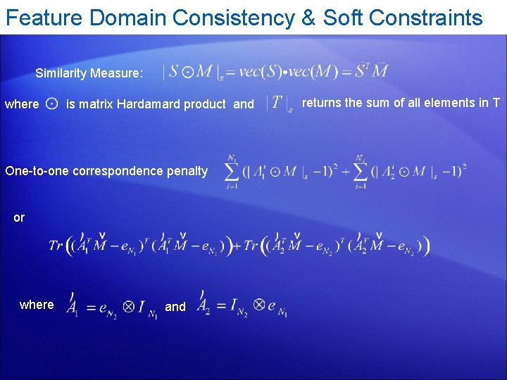
Feature Domain Consistency & Soft Constraints Similarity Measure: where is matrix Hardamard product and One-to-one correspondence penalty or where and returns the sum of all elements in T

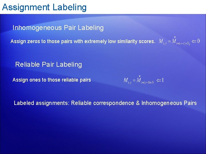
Assignment Labeling Inhomogeneous Pair Labeling Assign zeros to those pairs with extremely low similarity scores. Reliable Pair Labeling Assign ones to those reliable pairs Labeled assignments: Reliable correspondence & Inhomogeneous Pairs

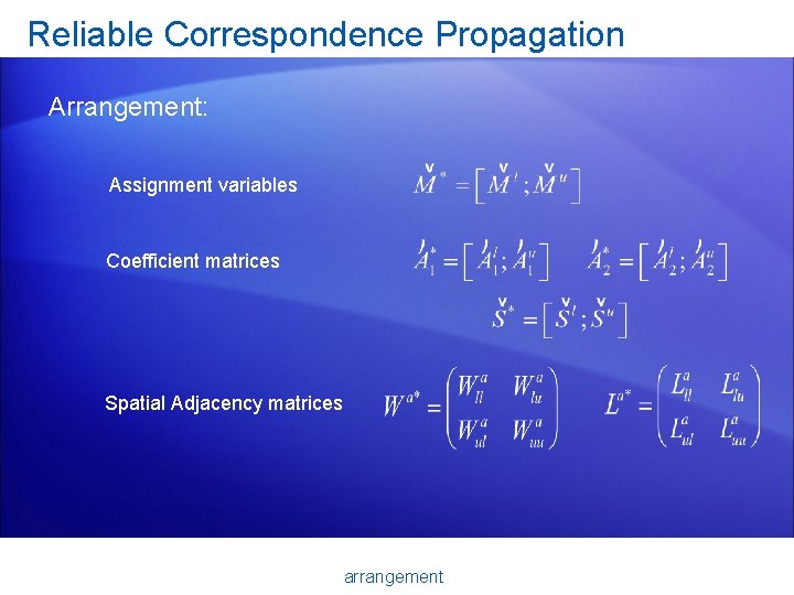
Reliable Correspondence Propagation Arrangement: Assignment variables Coefficient matrices Spatial Adjacency matrices arrangement

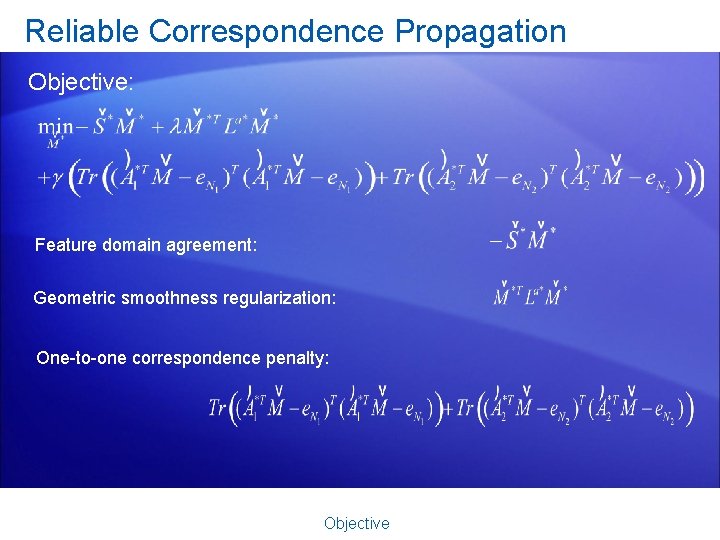
Reliable Correspondence Propagation Objective: Feature domain agreement: Geometric smoothness regularization: One-to-one correspondence penalty: Objective

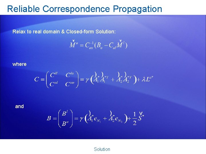
Reliable Correspondence Propagation Relax to real domain & Closed-form Solution: where and Solution

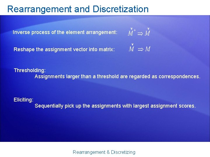
Rearrangement and Discretization Inverse process of the element arrangement: Reshape the assignment vector into matrix: Thresholding: Assignments larger than a threshold are regarded as correspondences. Eliciting: Sequentially pick up the assignments with largest assignment scores. Rearrangement & Discretizing

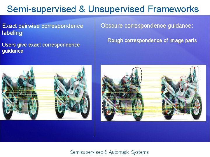
Semi-supervised & Unsupervised Frameworks Exact pairwise correspondence labeling: Users give exact correspondence guidance Obscure correspondence guidance: Rough correspondence of image parts Semisupervised & Automatic Systems

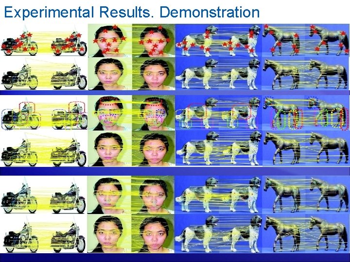
Experimental Results. Demonstration

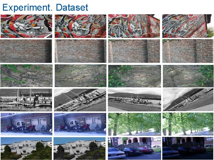
Experiment. Dataset

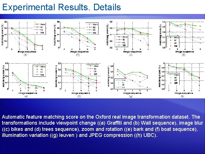
Experimental Results. Details Automatic feature matching score on the Oxford real image transformation dataset. The transformations include viewpoint change ((a) Graffiti and (b) Wall sequence), image blur ((c) bikes and (d) trees sequence), zoom and rotation ((e) bark and (f) boat sequence), illumination variation ((g) leuven ) and JPEG compression ((h) UBC).

Future Works • From point-to-point correspondence to set-to-set correspondence. • Multi-scale correspondence searching. Summary

Future Works • From point-to-point correspondence to set-to-set correspondence. • Multi-scale correspondence searching. • Combine the object segmentation and registration. Summary

Publications: [1] Huan Wang, Shuicheng Yan, Thomas Huang and Xiaoou Tang, ‘A convergent solution to Tensor Subspace Learning’, International Joint Conferences on Artificial Intelligence (IJCAI 07 Regular paper) , Jan. 2007. [2] Huan Wang, Shuicheng Yan, Thomas Huang and Xiaoou Tang, ‘Trace Ratio vs. Ratio Trace for Dimensionality Reduction’, IEEE Conference on Computer Vision and Pattern Recognition (CVPR 07), Jun. 2007. [3] Huan Wang, Shuicheng Yan, Thomas Huang, Jianzhuang Liu and Xiaoou Tang, ‘Transductive Regression Piloted by Inter-Manifold Relations ’, International Conference on Machine Learning (ICML 07), Jun. 2007. [4] Huan Wang, Shuicheng Yan, Thomas Huang and Xiaoou Tang, ‘Maximum unfolded embedding: formulation, solution, and application for image clustering ’, ACM international conference on Multimedia (ACM MM 07), Oct. 2006. [5] Shuicheng Yan, Huan Wang, Thomas Huang and Xiaoou Tang, ‘Ranking with Uncertain Labels ’, IEEE International Conference on Multimedia & Expo (ICME 07), May. 2007. [6] Shuicheng Yan, Huan Wang, Xiaoou Tang and Thomas Huang, ‘Exploring Feature Descriptors for Face Recognition ’, IEEE International Conference on Acoustics, Speech, and Signal Processing (ICASSP 07 Oral), Apri. 2007. Publications

Thank You!

Explore the intrinsic feature structures w. r. t. different classes for regression Transductive Regression on Multi-Class Data

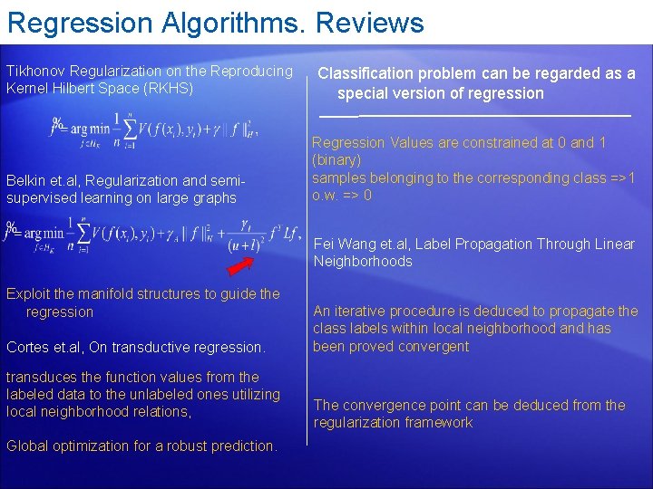
Regression Algorithms. Reviews Tikhonov Regularization on the Reproducing Kernel Hilbert Space (RKHS) Belkin et. al, Regularization and semisupervised learning on large graphs Classification problem can be regarded as a special version of regression Regression Values are constrained at 0 and 1 (binary) samples belonging to the corresponding class =>1 o. w. => 0 Fei Wang et. al, Label Propagation Through Linear Neighborhoods Exploit the manifold structures to guide the regression Cortes et. al, On transductive regression. transduces the function values from the labeled data to the unlabeled ones utilizing local neighborhood relations, Global optimization for a robust prediction. An iterative procedure is deduced to propagate the class labels within local neighborhood and has been proved convergent The convergence point can be deduced from the regularization framework

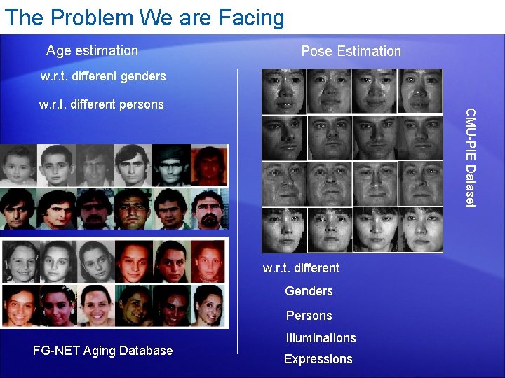
The Problem We are Facing Age estimation Pose Estimation w. r. t. different genders CMU-PIE Dataset w. r. t. different persons w. r. t. different Genders Persons FG-NET Aging Database Illuminations Expressions

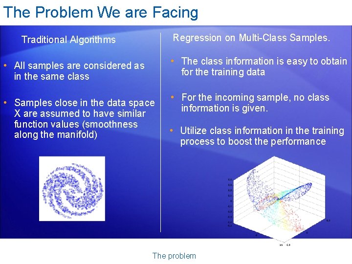
The Problem We are Facing Regression on Multi-Class Samples. Traditional Algorithms • The class information is easy to obtain for the training data • All samples are considered as in the same class • Samples close in the data space X are assumed to have similar function values (smoothness along the manifold) • For the incoming sample, no class information is given. • Utilize class information in the training process to boost the performance The problem

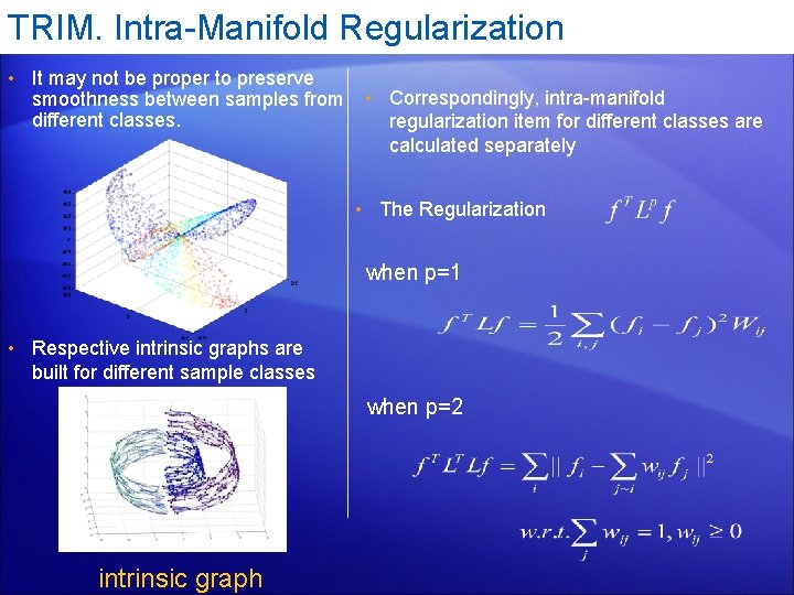
TRIM. Intra-Manifold Regularization • It may not be proper to preserve smoothness between samples from different classes. • Correspondingly, intra-manifold regularization item for different classes are calculated separately • The Regularization when p=1 • Respective intrinsic graphs are built for different sample classes when p=2 intrinsic graph

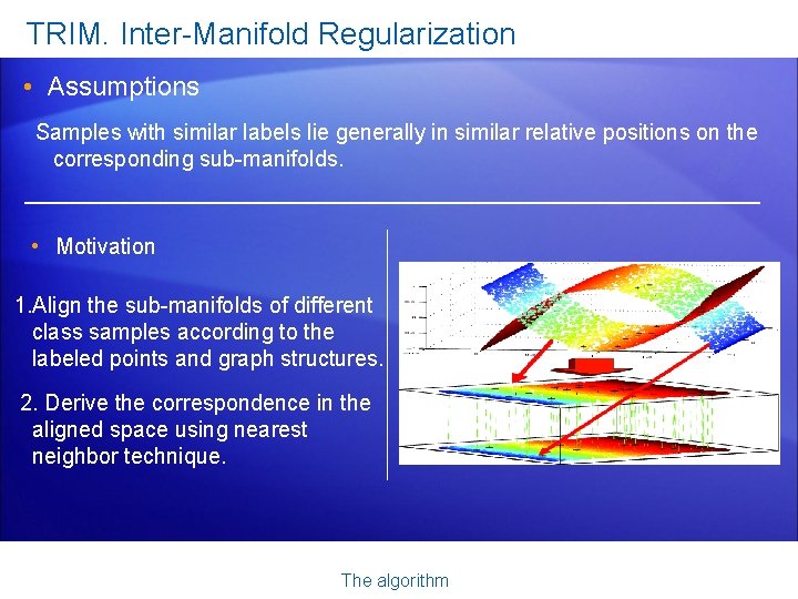
TRIM. Inter-Manifold Regularization • Assumptions Samples with similar labels lie generally in similar relative positions on the corresponding sub-manifolds. • Motivation 1. Align the sub-manifolds of different class samples according to the labeled points and graph structures. 2. Derive the correspondence in the aligned space using nearest neighbor technique. The algorithm

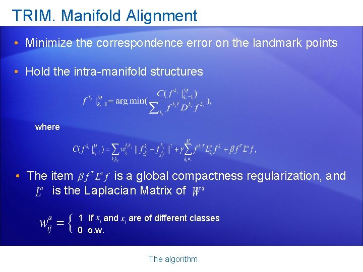
TRIM. Manifold Alignment • Minimize the correspondence error on the landmark points • Hold the intra-manifold structures where • The item is a global compactness regularization, and is the Laplacian Matrix of 1 If and 0 o. w. are of different classes The algorithm

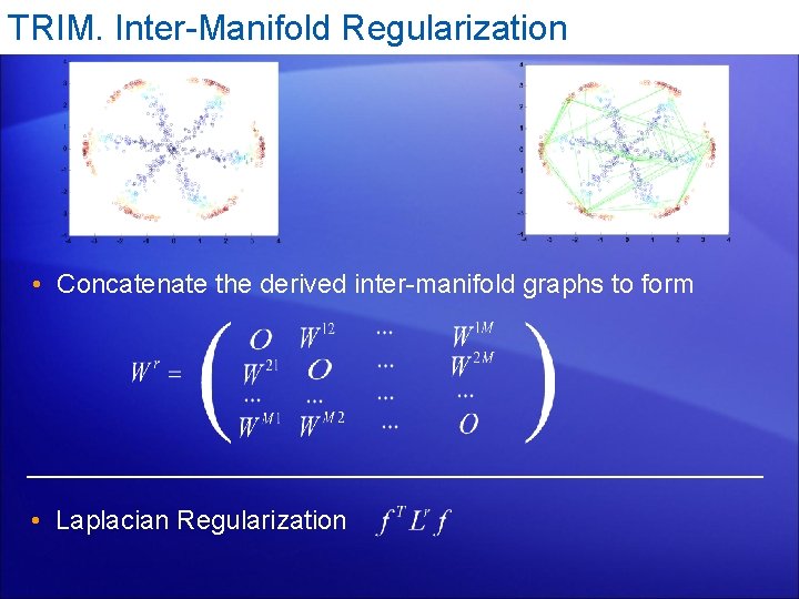
TRIM. Inter-Manifold Regularization • Concatenate the derived inter-manifold graphs to form • Laplacian Regularization

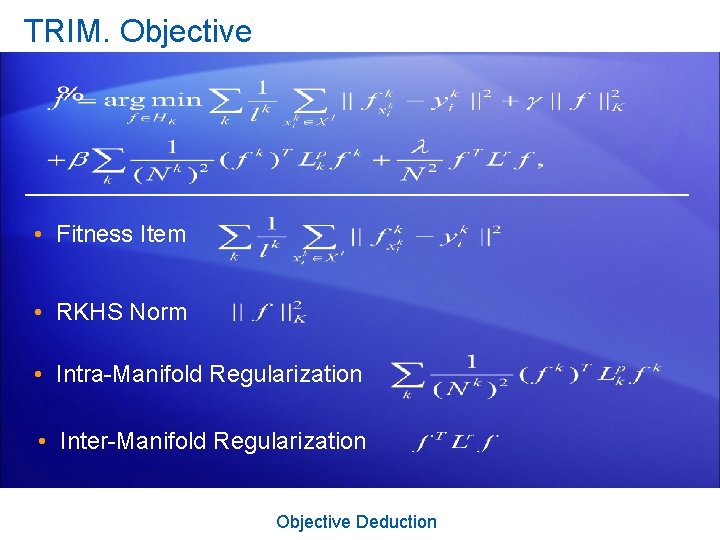
TRIM. Objective • Fitness Item • RKHS Norm • Intra-Manifold Regularization • Inter-Manifold Regularization Objective Deduction

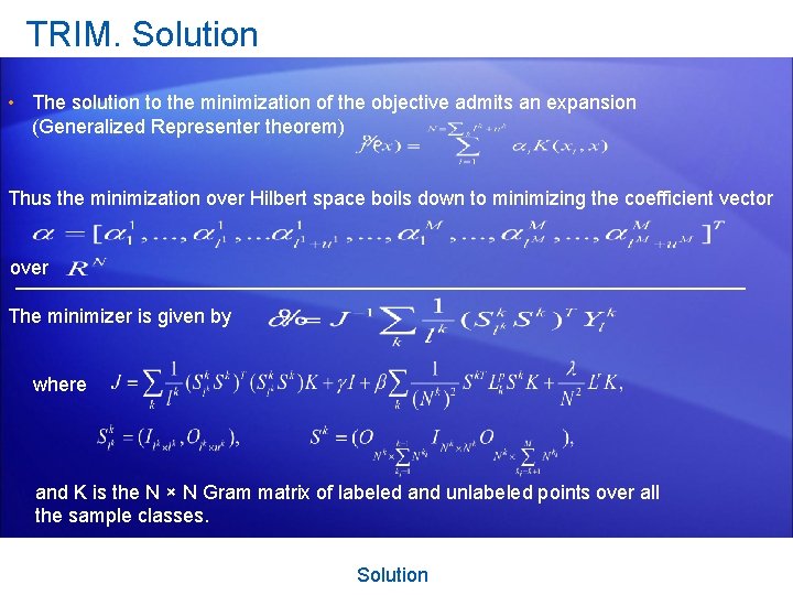
TRIM. Solution • The solution to the minimization of the objective admits an expansion (Generalized Representer theorem) Thus the minimization over Hilbert space boils down to minimizing the coefficient vector over The minimizer is given by where and K is the N × N Gram matrix of labeled and unlabeled points over all the sample classes. Solution

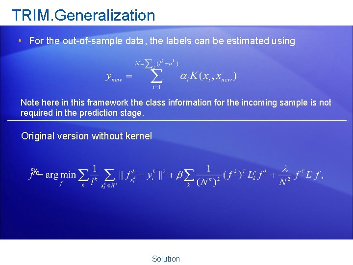
TRIM. Generalization • For the out-of-sample data, the labels can be estimated using Note here in this framework the class information for the incoming sample is not required in the prediction stage. Original version without kernel Solution

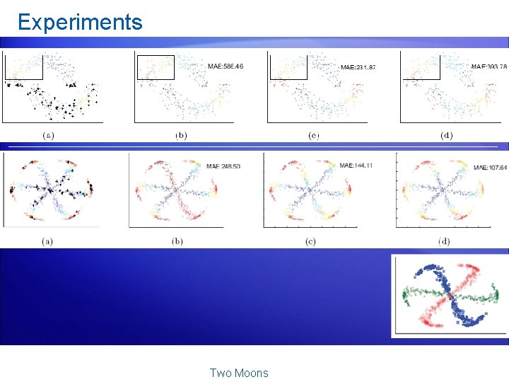
Experiments Two Moons

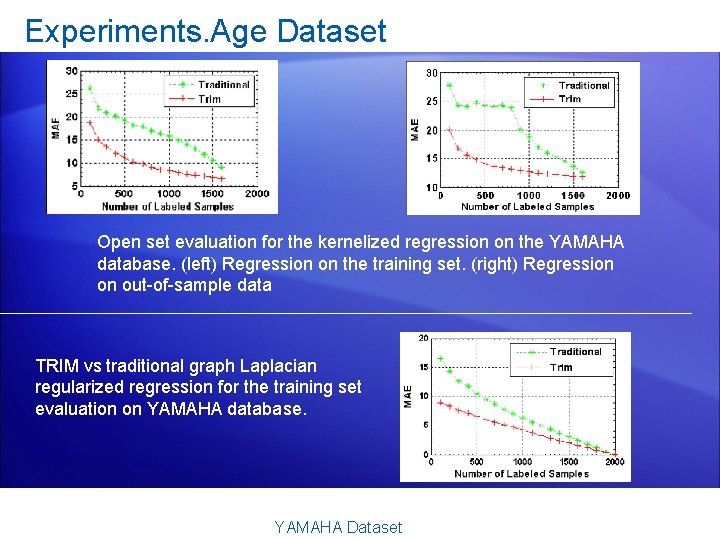
Experiments. Age Dataset Open set evaluation for the kernelized regression on the YAMAHA database. (left) Regression on the training set. (right) Regression on out-of-sample data TRIM vs traditional graph Laplacian regularized regression for the training set evaluation on YAMAHA database. YAMAHA Dataset