Exploring EDA Clustering and Data Preprocessing Lecture 1

Exploring EDA, Clustering and Data Preprocessing Lecture 1 Exploring EDA Vincent Croft NIKHEF - Nijmegen Inverted CERN School of Computing, 23 -24 February 2015 1 i. CSC 2015, Vince Croft, NIKHEF -Nijmegen

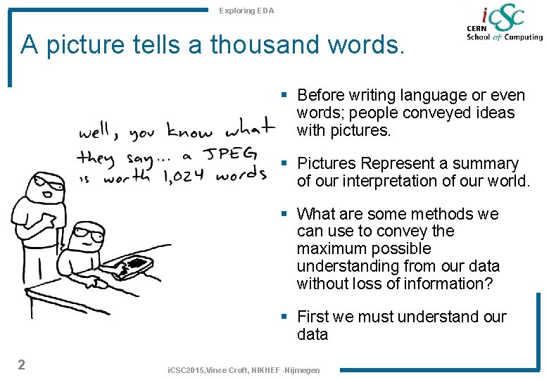
Exploring EDA A picture tells a thousand words. § Before writing language or even words; people conveyed ideas with pictures. § Pictures Represent a summary of our interpretation of our world. § What are some methods we can use to convey the maximum possible understanding from our data without loss of information? § First we must understand our data 2 i. CSC 2015, Vince Croft, NIKHEF -Nijmegen

Exploring EDA Probability vs. Statistics § Not the same thing… § Probability teaches us how to win big money in casinos. § Statistics shows that people don’t win big money in casinos. § Statistics is how we learn from past experiences § Exploratory Data Analysis is concerned with how to best learn from what data we have. 3 i. CSC 2015, Vince Croft, NIKHEF -Nijmegen

Exploring EDA Summary of things to come. § Visualization Basics. § What does data look like? § Understanding variables and distributions. § Manipulating Data. § Range, outliers, binning. § Transformations. § Adding Variables § Extracting hidden information § Correlation, Covariance, Dependence § Intro to MVA § Adding more variables, more information, and a gateway to lecture 2 4 i. CSC 2015, Vince Croft, NIKHEF -Nijmegen

Exploring EDA This Lecture is Brought to you by the letter R § R is a free open source programming language for statistics and data visualisation. § Simpler to learn then other languages such as python but more versatile then point and click programs such as SPSS § Many lectures and tutorials on the subject of EDA use examples given in R 5 i. CSC 2015, Vince Croft, NIKHEF -Nijmegen

Exploring EDA Worked Examples § All examples will be available online § If you are not here in person or want to see the examples presented for yourself please see the support documentation on my institute web page. http: //www. nikhef. nl/~vcroft/exploring. EDA. pdf http: //www. nikhef. nl/~vcroft/taking. Raw. Data. Towards. Analysis. pdf 6 i. CSC 2015, Vince Croft, NIKHEF -Nijmegen

Exploring EDA Other Resources § Coursera § “Exploratory Data Analysis” by Roger D. Peng, Ph. D, Jeff Leek, Ph. D, Brian Caffo, Ph. D § Udacity § “Data Analysis with R” by Facebook § Udacity § Intro to Hadoop and Map. Reduce by cloudera § Methods of Multivariate Analysis § Alvin C Rencher 7 i. CSC 2015, Vince Croft, NIKHEF -Nijmegen

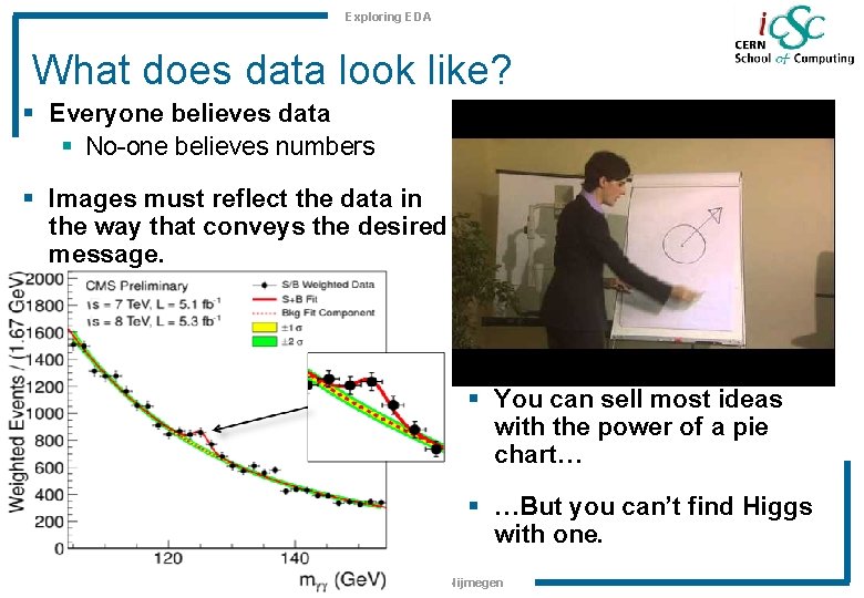
Exploring EDA What does data look like? § Everyone believes data § No-one believes numbers § Images must reflect the data in the way that conveys the desired message. § You can sell most ideas with the power of a pie chart… § …But you can’t find Higgs with one. 8 i. CSC 2015, Vince Croft, NIKHEF -Nijmegen

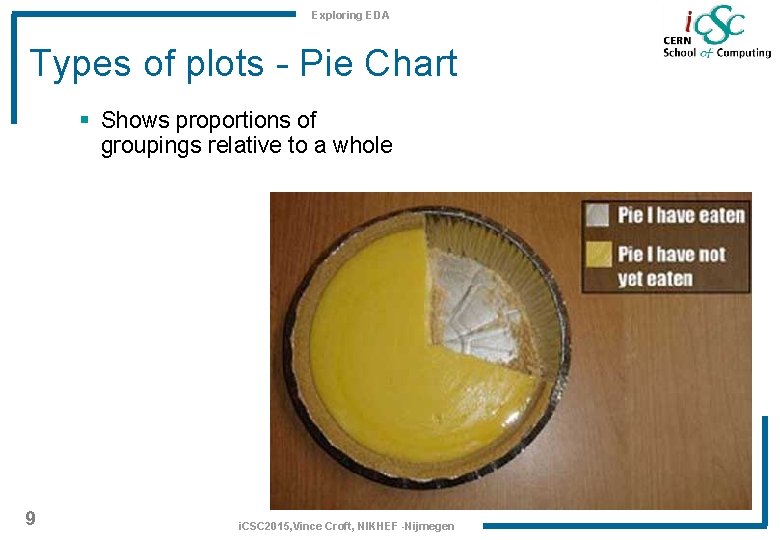
Exploring EDA Types of plots - Pie Chart § Shows proportions of groupings relative to a whole 9 i. CSC 2015, Vince Croft, NIKHEF -Nijmegen

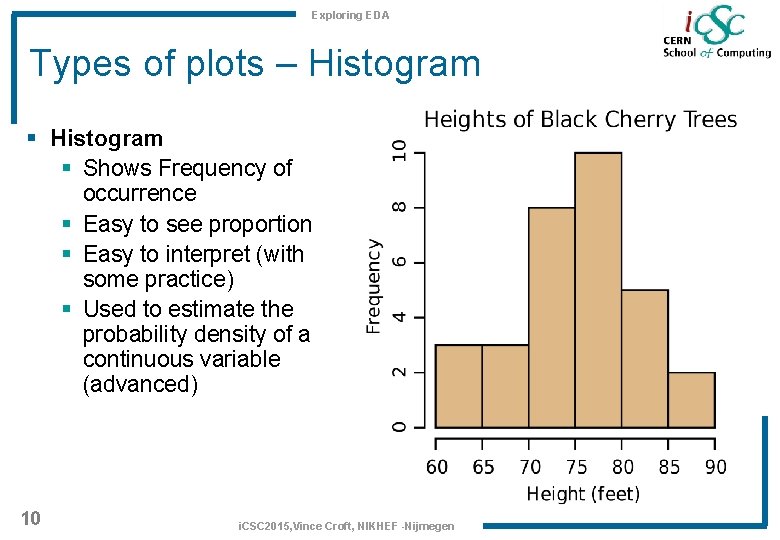
Exploring EDA Types of plots – Histogram § Shows Frequency of occurrence § Easy to see proportion § Easy to interpret (with some practice) § Used to estimate the probability density of a continuous variable (advanced) 10 i. CSC 2015, Vince Croft, NIKHEF -Nijmegen

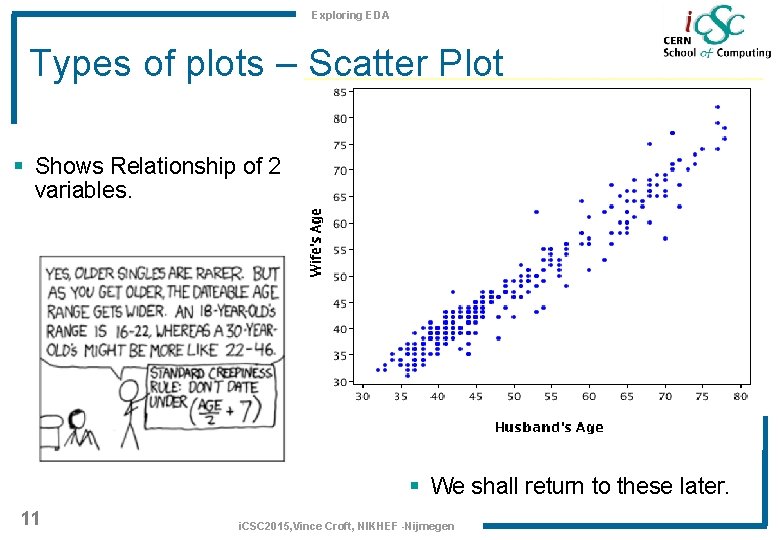
Exploring EDA Types of plots – Scatter Plot § Shows Relationship of 2 variables. § We shall return to these later. 11 i. CSC 2015, Vince Croft, NIKHEF -Nijmegen

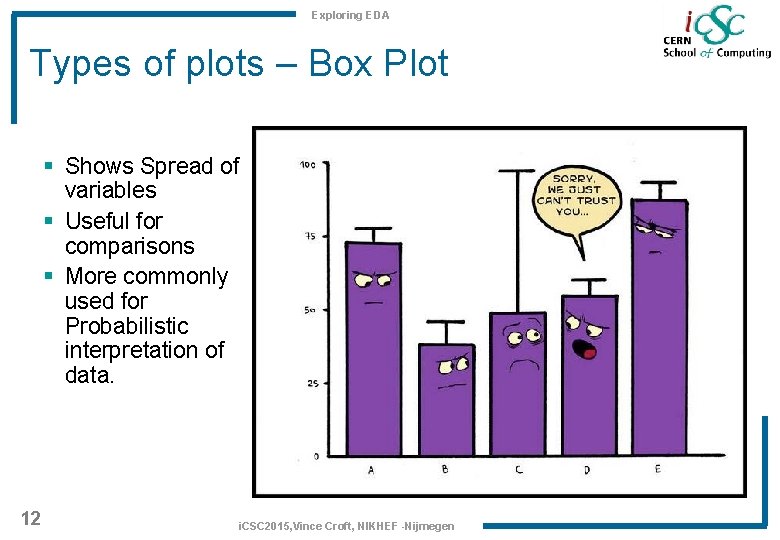
Exploring EDA Types of plots – Box Plot § Shows Spread of variables § Useful for comparisons § More commonly used for Probabilistic interpretation of data. 12 i. CSC 2015, Vince Croft, NIKHEF -Nijmegen

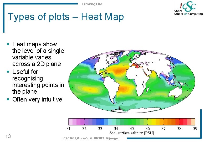
Exploring EDA Types of plots – Heat Map § Heat maps show the level of a single variable varies across a 2 D plane § Useful for recognising interesting points in the plane § Often very intuitive 13 i. CSC 2015, Vince Croft, NIKHEF -Nijmegen

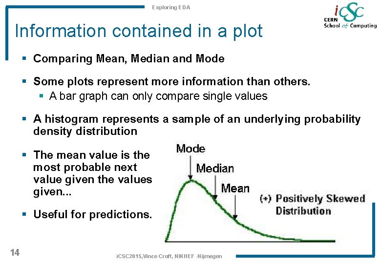
Exploring EDA Information contained in a plot § Comparing Mean, Median and Mode § Some plots represent more information than others. § A bar graph can only compare single values § A histogram represents a sample of an underlying probability density distribution § The mean value is the most probable next value given the values given. . . § Useful for predictions. 14 i. CSC 2015, Vince Croft, NIKHEF -Nijmegen

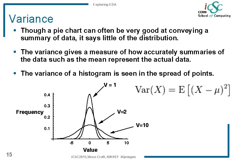
Exploring EDA Variance § Though a pie chart can often be very good at conveying a summary of data, it says little of the distribution. § The variance gives a measure of how accurately summaries of the data such as the mean represent the actual data. § The variance of a histogram is seen in the spread of points. 15 i. CSC 2015, Vince Croft, NIKHEF -Nijmegen

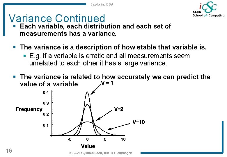
Exploring EDA Variance Continued § Each variable, each distribution and each set of measurements has a variance. § The variance is a description of how stable that variable is. § E. g. if a variable is erratic and all measurements seem unrelated to each other it has a large variance. § The variance is related to how accurately we can predict the value of a variable 16 i. CSC 2015, Vince Croft, NIKHEF -Nijmegen

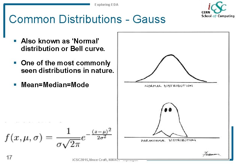
Exploring EDA Common Distributions - Gauss § Also known as ‘Normal’ distribution or Bell curve. § One of the most commonly seen distributions in nature. § Mean=Median=Mode 17 i. CSC 2015, Vince Croft, NIKHEF -Nijmegen

Exploring EDA Common Distributions - Exponential § Commonly seen in lifetimes. § Represents the time between two independent and random events. § Memoryless § A good model for many things from radioactive decay to requests for documents on a web server. 18 i. CSC 2015, Vince Croft, NIKHEF -Nijmegen

Exploring EDA Displaying your data § Range – focus on interesting features § Binning – What represents the data best? § Error in measurement § More bins then possible values? 19 i. CSC 2015, Vince Croft, NIKHEF -Nijmegen

Exploring EDA Noise – Bias – Sampling Error § If a graph looks noisy, most likely you have too many bins for the data you’re plotting § Using too few bins increases likelihood of introducing a bias (plot doesn’t represent the true distribution) § Variance is a measure of how well we can predict a value. If we hide this feature of the data by increasing bin size then we risk loosing information. § Noise or Variance? It’s sometimes a tough decision! 20 i. CSC 2015, Vince Croft, NIKHEF -Nijmegen

Exploring EDA Transformations § Division – Binning § You can scale one axis or change the binning. § You can divide all values by another set of values… § Log Scale § y – focus on interesting features that happen in tails of the distribution § Others § Square Root § 1/x 21 i. CSC 2015, Vince Croft, NIKHEF -Nijmegen

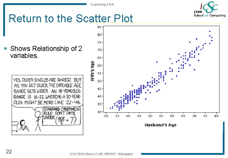
Exploring EDA Return to the Scatter Plot § Shows Relationship of 2 variables. 22 i. CSC 2015, Vince Croft, NIKHEF -Nijmegen

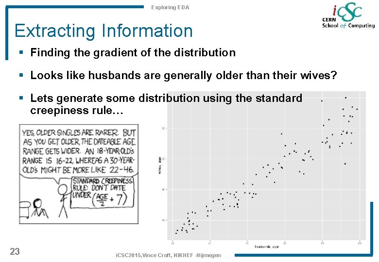
Exploring EDA Extracting Information § Finding the gradient of the distribution § Looks like husbands are generally older than their wives? § Lets generate some distribution using the standard creepiness rule… 23 i. CSC 2015, Vince Croft, NIKHEF -Nijmegen

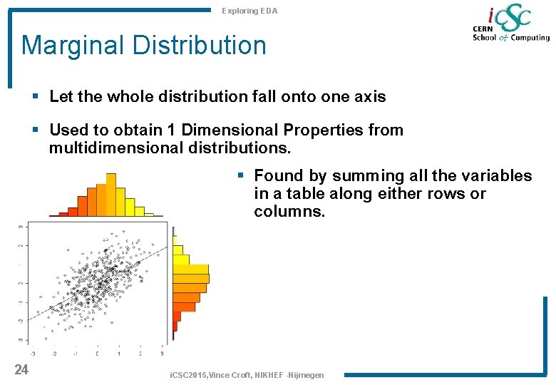
Exploring EDA Marginal Distribution § Let the whole distribution fall onto one axis § Used to obtain 1 Dimensional Properties from multidimensional distributions. § Found by summing all the variables in a table along either rows or columns. 24 i. CSC 2015, Vince Croft, NIKHEF -Nijmegen

Exploring EDA 2 D Transformations § If we think of variables as measurements taken from a certain position, transformations can be used to see measurements from a different perspective. § Useful information can be extracted from the transformed distribution. § Transformed variables might have some physical meaning or demonstrate some interesting feature. 25 i. CSC 2015, Vince Croft, NIKHEF -Nijmegen

Exploring EDA Correlation and Covariance § Correlation and covariance is the degree to which we expect one variable to behave given the action of another. § e. g. taller people usually weigh more. Therefore human height and weight co-vary and are correlated § Both Correlation and Covariance describe the deviation of variables away from the mean § Covariance depends on the scale of the measurement. Has units! § Correlation is a standardised covariance such that it can be measured between -1 and 1 without units. 26 i. CSC 2015, Vince Croft, NIKHEF -Nijmegen

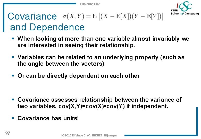
Exploring EDA Covariance and Dependence § When looking at more than one variable almost invariably we are interested in seeing their relationship. § Variables can be related to an underlying property (such as the angle between the vectors) § Or can be directly dependent on each other § Covariance assesses relationship between the variance of two variables. cov(X, Y)=cov(X) cov(Y) if independent. § Covariance has units! 27 i. CSC 2015, Vince Croft, NIKHEF -Nijmegen

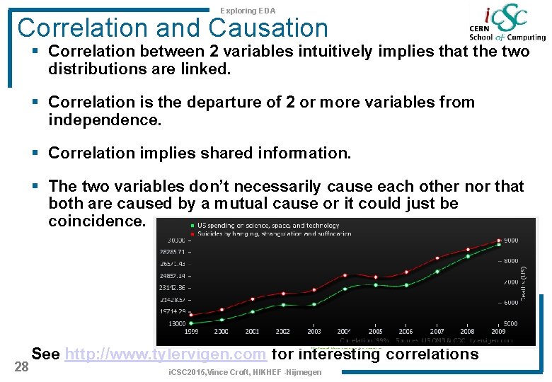
Exploring EDA Correlation and Causation § Correlation between 2 variables intuitively implies that the two distributions are linked. § Correlation is the departure of 2 or more variables from independence. § Correlation implies shared information. § The two variables don’t necessarily cause each other nor that both are caused by a mutual cause or it could just be coincidence. 28 See http: //www. tylervigen. com for interesting correlations i. CSC 2015, Vince Croft, NIKHEF -Nijmegen

Exploring EDA Characterising 2 D Data § 2 Variables such as X and Y can be considered as two vectors of measurements. § These vectors can be mapped to the x and y axis of a scatter plot. § The means and variances of each can be extracted from the marginal distributions of this plot § The correlation between these plots can be understood as the cosine of the angle between the vectors X and Y 29 i. CSC 2015, Vince Croft, NIKHEF -Nijmegen

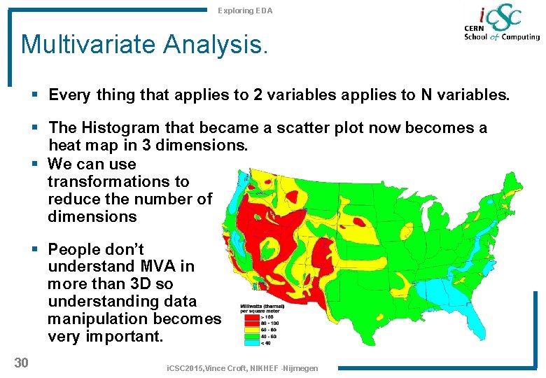
Exploring EDA Multivariate Analysis. § Every thing that applies to 2 variables applies to N variables. § The Histogram that became a scatter plot now becomes a heat map in 3 dimensions. § We can use transformations to reduce the number of dimensions § People don’t understand MVA in more than 3 D so understanding data manipulation becomes very important. 30 i. CSC 2015, Vince Croft, NIKHEF -Nijmegen