Exploration on statistical and timeseries models Jonathan Samama

Exploration on statistical and time-series models Jonathan Samama, Jonathan Horyn Julien Bect, Emmanuel Vazquez SUPELEC Cécile Germain-Renaud LRI

The problem: Statistical characterization and models of job arrival and components load Here component = CE 2

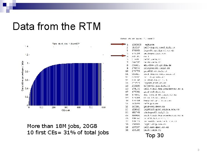
Data from the RTM More than 18 M jobs, 20 GB 10 first CEs= 31% of total jobs Top 30 3

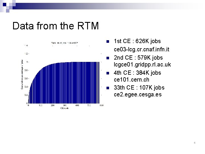
Data from the RTM n n 1 st CE : 626 K jobs ce 03 -lcg. cr. cnaf. infn. it 2 nd CE : 579 K jobs lcgce 01. gridpp. rl. ac. uk 4 th CE : 384 K jobs ce 101. cern. ch 33 th CE : 107 K jobs ce 2. egee. cesga. es 4

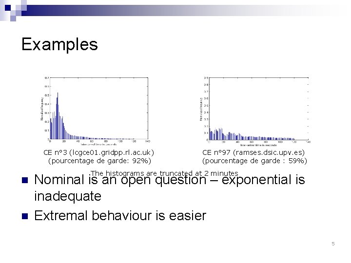
Examples CE n° 3 (lcgce 01. gridpp. rl. ac. uk) (pourcentage de garde: 92%) n n CE n° 97 (ramses. dsic. upv. es) (pourcentage de garde : 59%) The histograms are truncated at 2 minutes Nominal is an open question – exponential is inadequate Extremal behaviour is easier 5

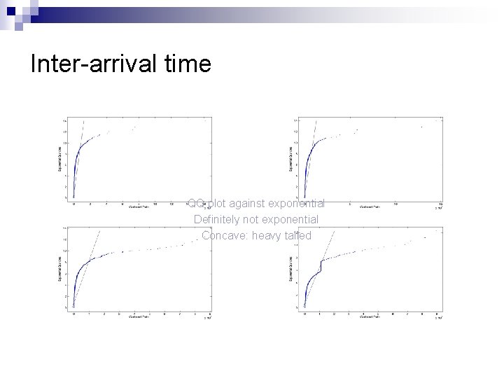
Inter-arrival time QQ plot against exponential Definitely not exponential Concave: heavy tailed

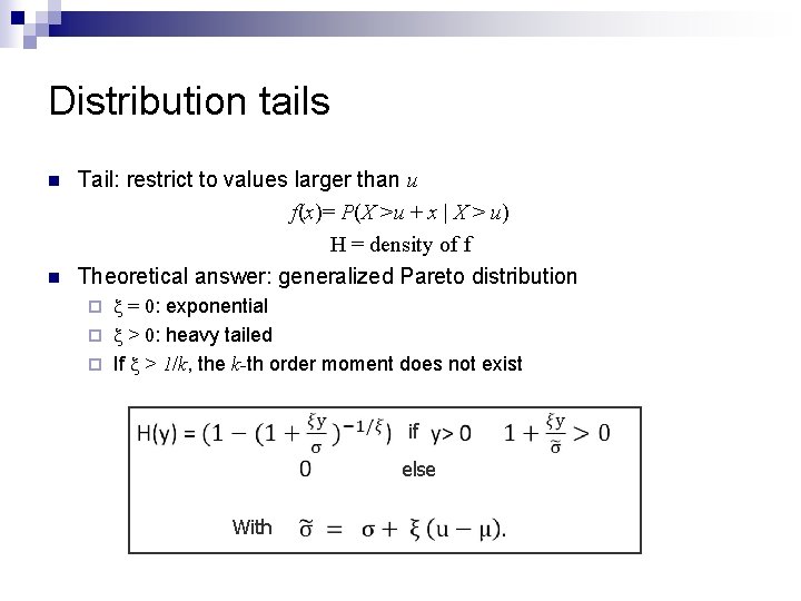
Distribution tails n n Tail: restrict to values larger than u f(x)= P(X >u + x | X > u) H = density of f Theoretical answer: generalized Pareto distribution x = 0: exponential ¨ x > 0: heavy tailed ¨ If x > 1/k, the k-th order moment does not exist ¨ if else With

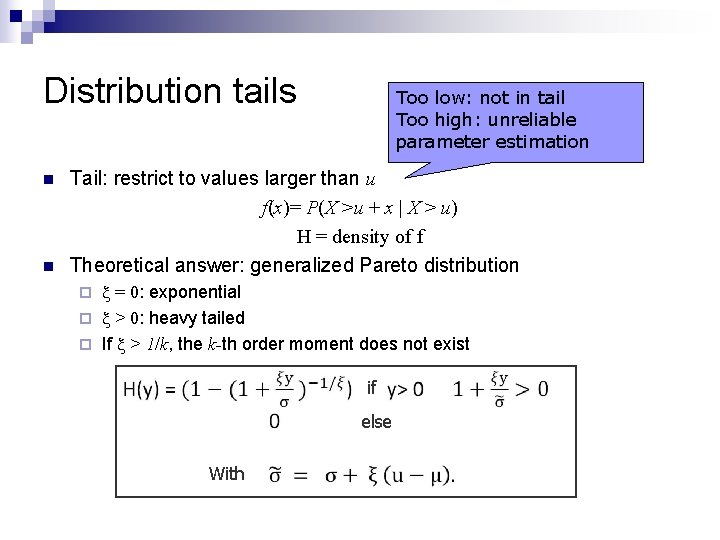
Distribution tails n n Too low: not in tail Too high: unreliable parameter estimation Tail: restrict to values larger than u f(x)= P(X >u + x | X > u) H = density of f Theoretical answer: generalized Pareto distribution x = 0: exponential ¨ x > 0: heavy tailed ¨ If x > 1/k, the k-th order moment does not exist ¨ if else With

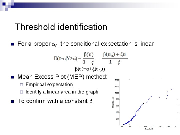
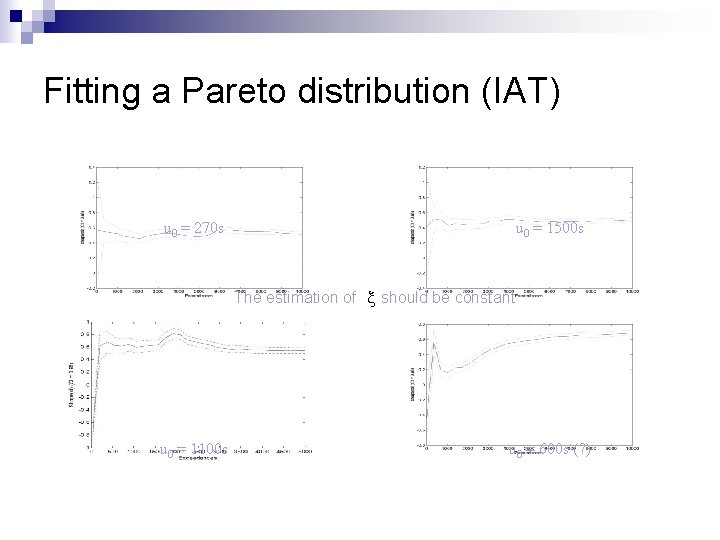
Threshold identification n For a proper u 0, the conditional expectation is linear b(u)=s+x(u-m) n Mean Excess Plot (MEP) method: Empirical expectation ¨ Identify a linear area in the graph ¨ n To confirm with a constant x 9

Fitting a Pareto distribution (IAT) u 0 = 270 s u 0 = 1500 s The estimation of x should be constant u 0 = 1100 s u 0 = 600 s (? )

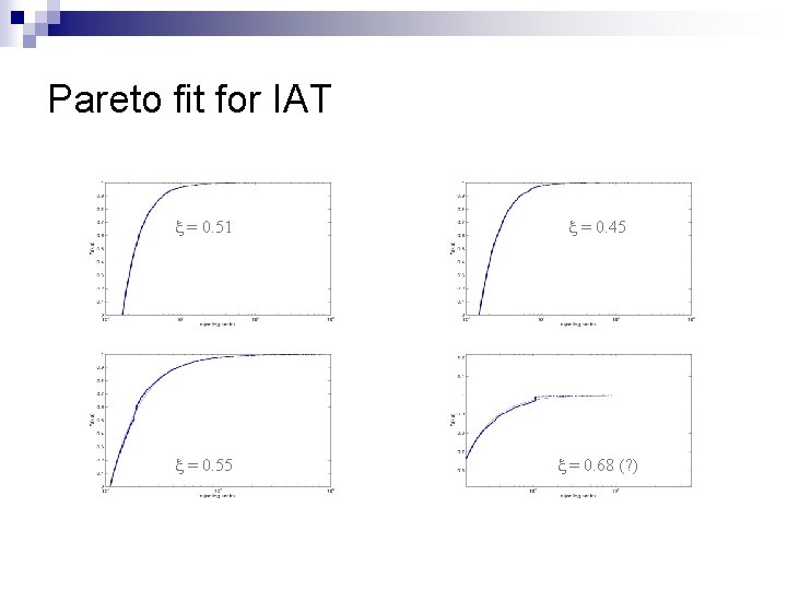
Pareto fit for IAT x = 0. 51 x = 0. 45 x = 0. 55 x = 0. 68 (? )

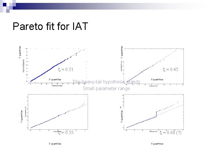
Y quantiles Pareto fit for IAT x = 0. 51 X quantiles Y quantiles The heavy-tail hypothesis stands Small parameter range Y quantiles X quantiles x = 0. 45 x = 0. 55 X quantiles x = 0. 68 (? ) X quantiles

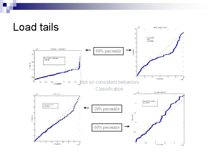
Load tails 90% percentile Not so consistent behaviors Classification 20% percentile 60% percentile

Are statistics relevant? v Arrival process intensity v Inverse of the average IAT v Average range: day, week v Stationarity v Intensity (and average) do not depend on date v Poisson process (exponential IAT) are stationary 14

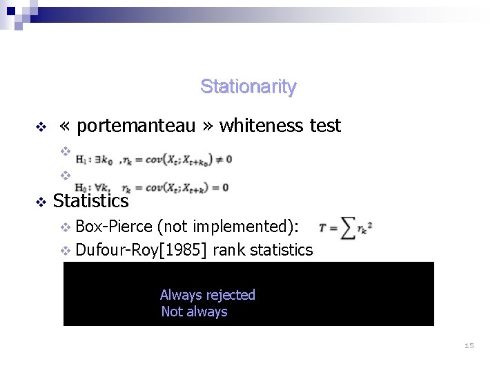
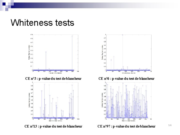
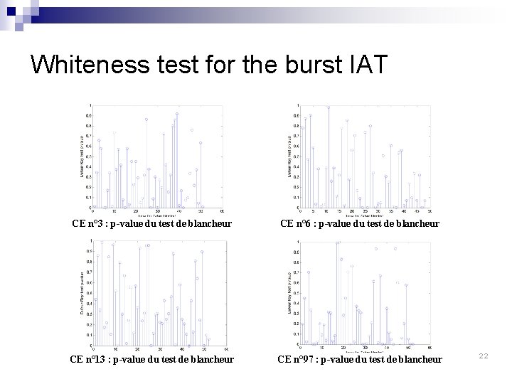
Stationarity v « portemanteau » whiteness test v v v Statistics v Box-Pierce (not implemented): v Dufour-Roy[1985] rank statistics At the day scale Always rejected on active CEs Not always on less active CEs 15

Whiteness tests CE n° 3 : p-value du test de blancheur CE n° 6 : p-value du test de blancheur CE n° 13 : p-value du test de blancheur CE n° 97 : p-value du test de blancheur 16

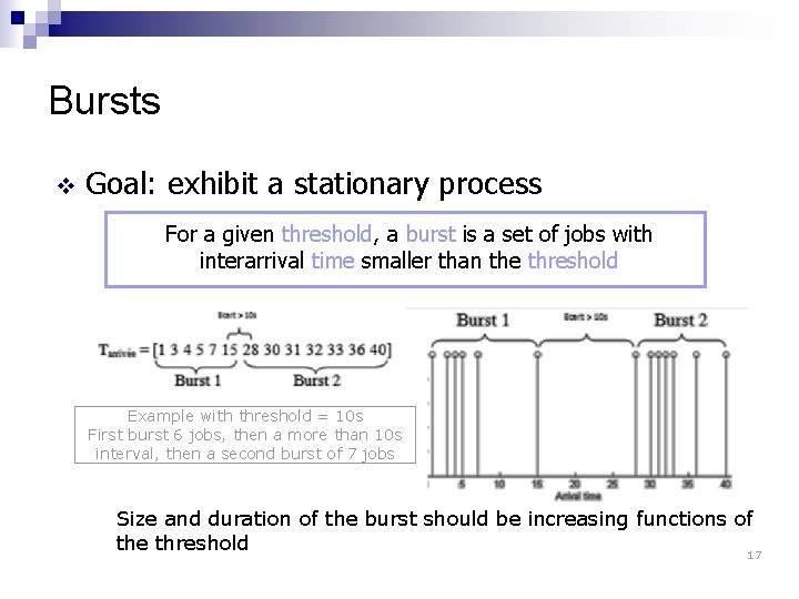
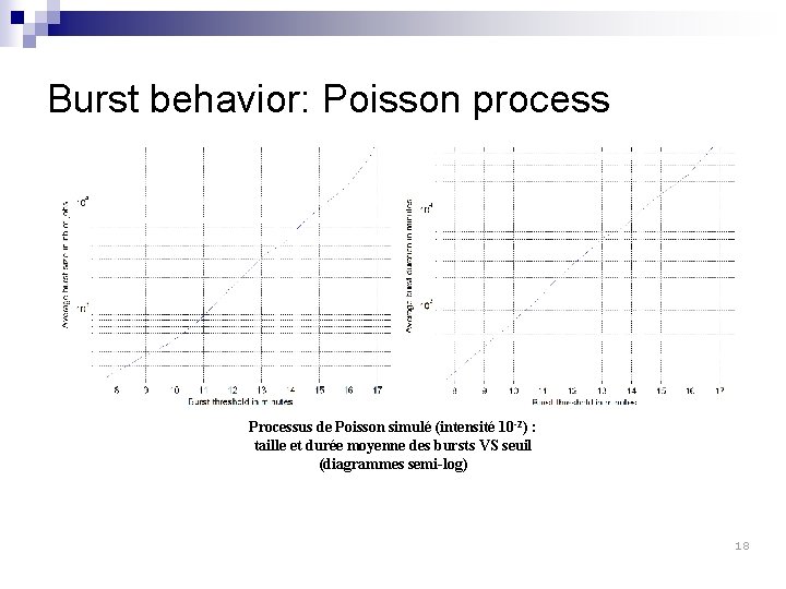
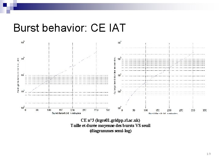
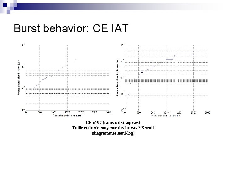
Bursts v Goal: exhibit a stationary process For a given threshold, a burst is a set of jobs with interarrival time smaller than the threshold Example with threshold = 10 s First burst 6 jobs, then a more than 10 s interval, then a second burst of 7 jobs Size and duration of the burst should be increasing functions of the threshold 17

Burst behavior: Poisson process Processus de Poisson simulé (intensité 10 -2) : taille et durée moyenne des bursts VS seuil (diagrammes semi-log) 18

Burst behavior: CE IAT CE n° 3 (lcgce 01. gridpp. rl. ac. uk) Taille et durée moyenne des bursts VS seuil (diagrammes semi-log) 19

Burst behavior: CE IAT CE n° 97 (ramses. dsic. upv. es) Taille et durée moyenne des bursts VS seuil (diagrammes semi-log)

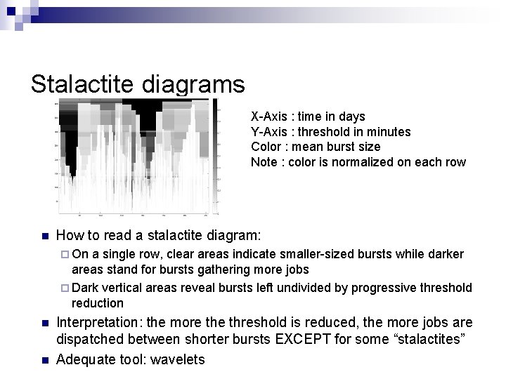
Burst intensity Reciprocal of the mean IAT of the bursts n The independence hypothesis of the IAT is not systematically rejected even on the most active CEs n At the week scale n 21

Whiteness test for the burst IAT CE n° 3 : p-value du test de blancheur CE n° 6 : p-value du test de blancheur CE n° 13 : p-value du test de blancheur CE n° 97 : p-value du test de blancheur 22

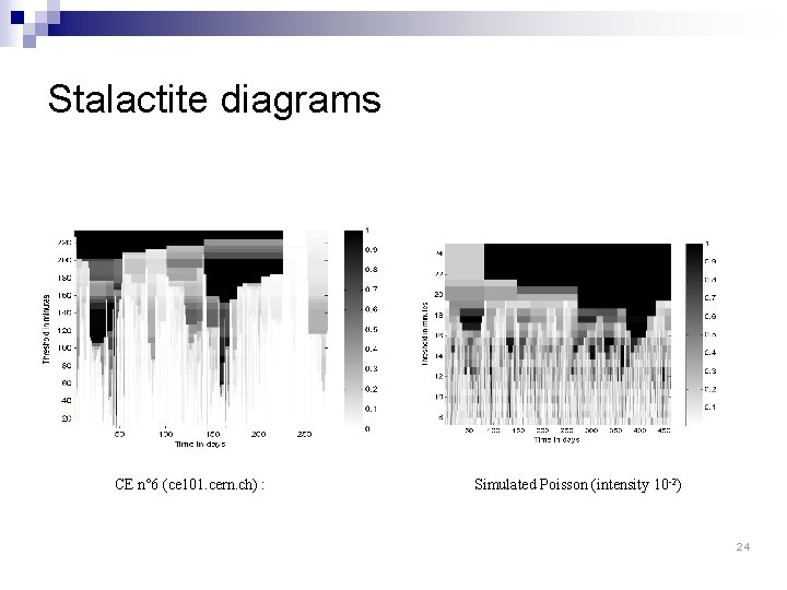
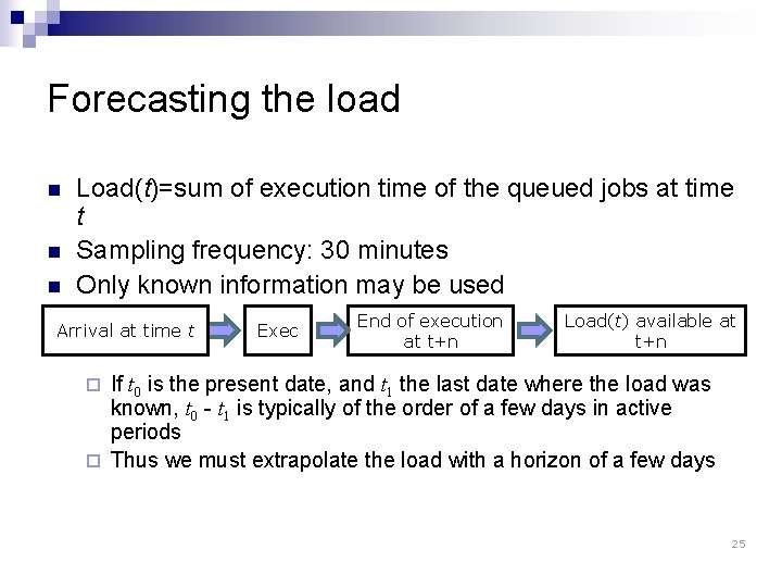
Stalactite diagrams X-Axis : time in days Y-Axis : threshold in minutes Color : mean burst size Note : color is normalized on each row n How to read a stalactite diagram: ¨ On a single row, clear areas indicate smaller-sized bursts while darker areas stand for bursts gathering more jobs ¨ Dark vertical areas reveal bursts left undivided by progressive threshold reduction n n Interpretation: the more threshold is reduced, the more jobs are dispatched between shorter bursts EXCEPT for some “stalactites” Adequate tool: wavelets

Stalactite diagrams CE n° 6 (ce 101. cern. ch) : Simulated Poisson (intensity 10 -2) 24

Forecasting the load n n n Load(t)=sum of execution time of the queued jobs at time t Sampling frequency: 30 minutes Only known information may be used Arrival at time t Exec End of execution at t+n Load(t) available at t+n If t 0 is the present date, and t 1 the last date where the load was known, t 0 - t 1 is typically of the order of a few days in active periods ¨ Thus we must extrapolate the load with a horizon of a few days ¨ 25

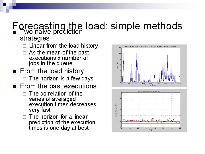
Forecasting the load: simple methods n Two naive prediction strategies ¨ ¨ n From the load history ¨ n Linear from the load history As the mean of the past executions x number of jobs in the queue The horizon is a few days From the past executions The correlation of the series of averaged execution times decreases very fast ¨ The horizon for a linear prediction of the execution times is one day at best ¨

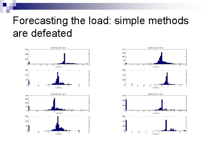
Forecasting the load: simple methods are defeated

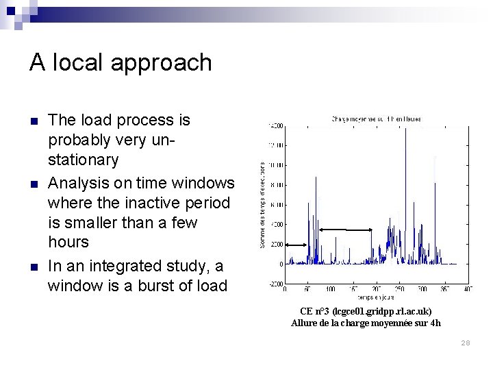
A local approach n n n The load process is probably very unstationary Analysis on time windows where the inactive period is smaller than a few hours In an integrated study, a window is a burst of load CE n° 3 (lcgce 01. gridpp. rl. ac. uk) Allure de la charge moyennée sur 4 h 28

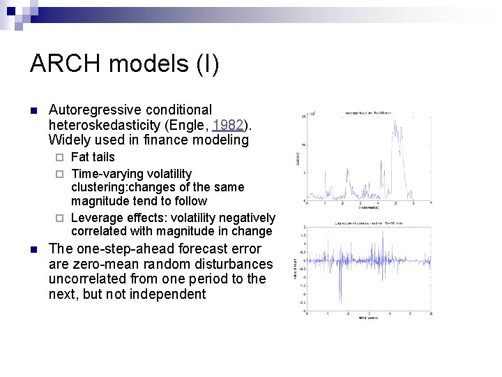
ARCH models (I) n Autoregressive conditional heteroskedasticity (Engle, 1982). Widely used in finance modeling Fat tails ¨ Time-varying volatility clustering: changes of the same magnitude tend to follow ¨ Leverage effects: volatility negatively correlated with magnitude in change ¨ n The one-step-ahead forecast error are zero-mean random disturbances uncorrelated from one period to the next, but not independent

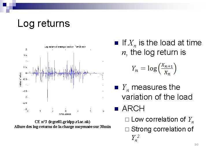
Log returns n If Xn is the load at time n, the log return is n Yn measures the variation of the load ARCH n CE n° 3 (lcgce 01. gridpp. rl. ac. uk) Allure des log-returns de la charge moyennée sur 30 min ¨ Low correlation of Yn ¨ Strong correlation of Yn 2 30

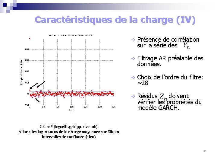
Caractéristiques de la charge (IV) v Présence de corrélation sur la série des . v Filtrage AR préalable des données. v Choix de l’ordre du filtre: ~28 v Résidus doivent vérifier les propriétés du modèle GARCH. CE n° 3 (lcgce 01. gridpp. rl. ac. uk) Allure des log-returns de la charge moyennée sur 30 min Intervalles de confiance (bleu) 31

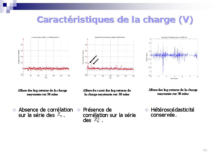
Caractéristiques de la charge (V) Allure des log-returns de la charge moyennée sur 30 mins v Allure du carré des log-returns de la charge moyénnée sur 30 mins Absence de corrélation v Présence de sur la série des . corrélation sur la série des . Allure des log-returns de la charge moyennée sur 30 mins v Hétéroscédasticité conservée. 32

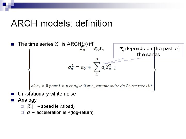
ARCH models: definition n The time series Zn is ARCH(p) iff sn depends on the past of the series n n Un-stationary white noise Analogy ¨ |Zn| ~ speed ie D(load) ¨ sn ~ acceleration ie D(log-return)

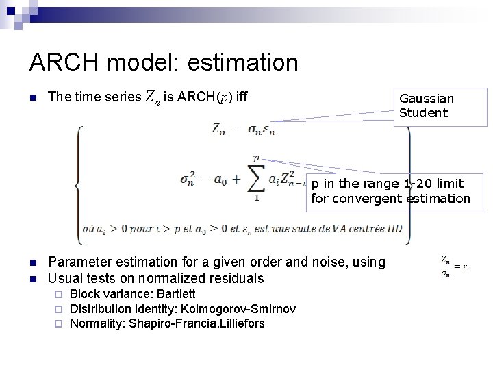
ARCH model: estimation n The time series Zn is ARCH(p) iff Gaussian Student p in the range 1 -20 limit for convergent estimation n n Parameter estimation for a given order and noise, using Usual tests on normalized residuals ¨ ¨ ¨ Block variance: Bartlett Distribution identity: Kolmogorov-Smirnov Normality: Shapiro-Francia, Lilliefors

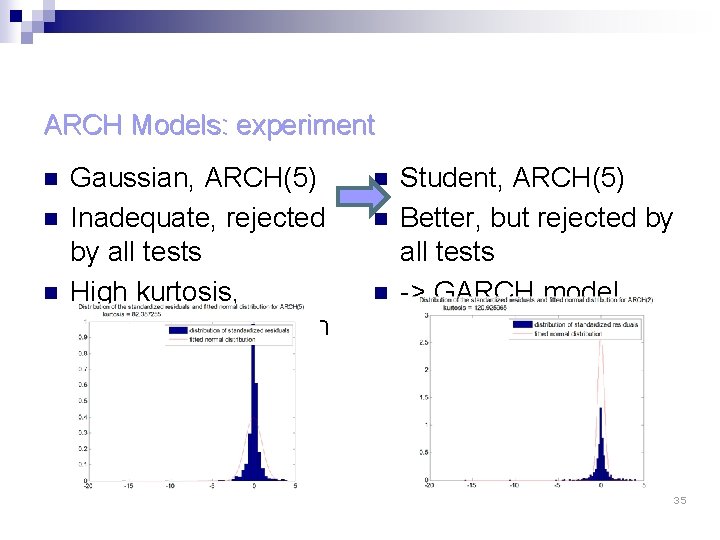
ARCH Models: experiment n n n Gaussian, ARCH(5) Inadequate, rejected by all tests High kurtosis, Student’s distribution n Student, ARCH(5) Better, but rejected by all tests -> GARCH model 35

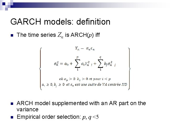
GARCH models: definition n The time series Zn is ARCH(p) iff n ARCH model supplemented with an AR part on the variance Empirical order selection: p, q <5 n

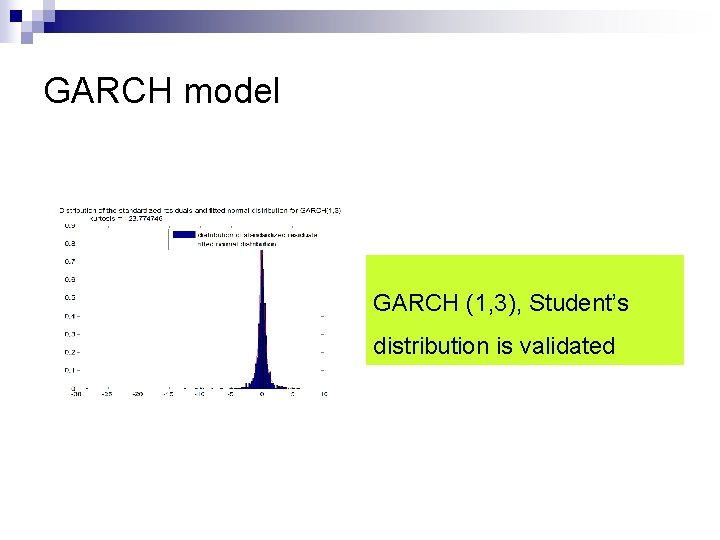
GARCH model GARCH (1, 3), Student’s distribution is validated

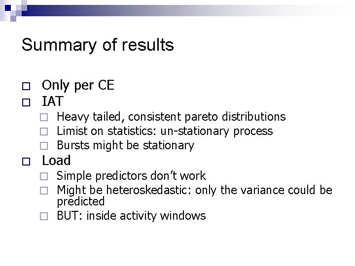
Summary of results � � Only per CE IAT � � Heavy tailed, consistent pareto distributions Limist on statistics: un-stationary process Bursts might be stationary Load Simple predictors don’t work Might be heteroskedastic: only the variance could be predicted � BUT: inside activity windows � �

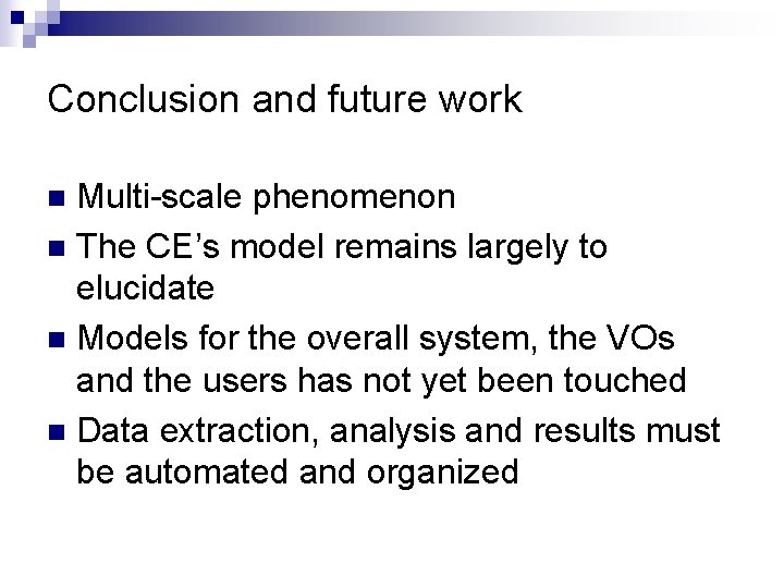
Conclusion and future work Multi-scale phenomenon n The CE’s model remains largely to elucidate n Models for the overall system, the VOs and the users has not yet been touched n Data extraction, analysis and results must be automated and organized n

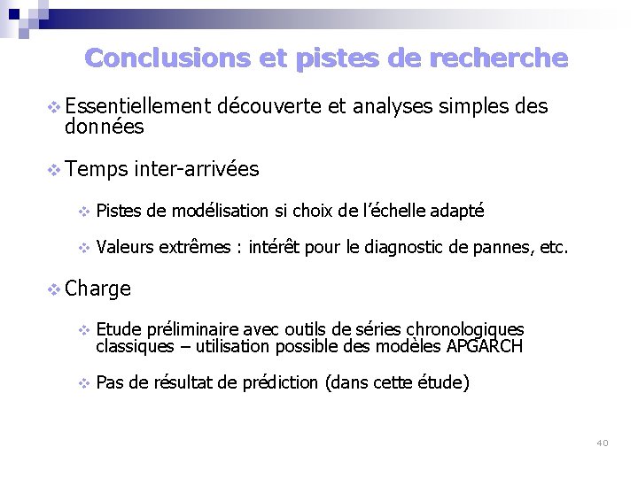
Conclusions et pistes de recherche v Essentiellement découverte et analyses simples des données v Temps inter-arrivées v Pistes de modélisation si choix de l’échelle adapté v Valeurs extrêmes : intérêt pour le diagnostic de pannes, etc. v Charge v Etude préliminaire avec outils de séries chronologiques classiques – utilisation possible des modèles APGARCH v Pas de résultat de prédiction (dans cette étude) 40