Explicit Computation of Performance as a Function of

Explicit Computation of Performance as a Function of Process Parameters Lou Scheffer 1 Tau 2002

What’s the problem? • Chip manufacturing not perfect, so…. • Each chip is different • Designers want as many chips as possible to work • We consider 3 kinds of variation ‑ Inter-chip ‑ Intra-chip ‣ Deterministic ‣ Statistical 2 Tau 2002

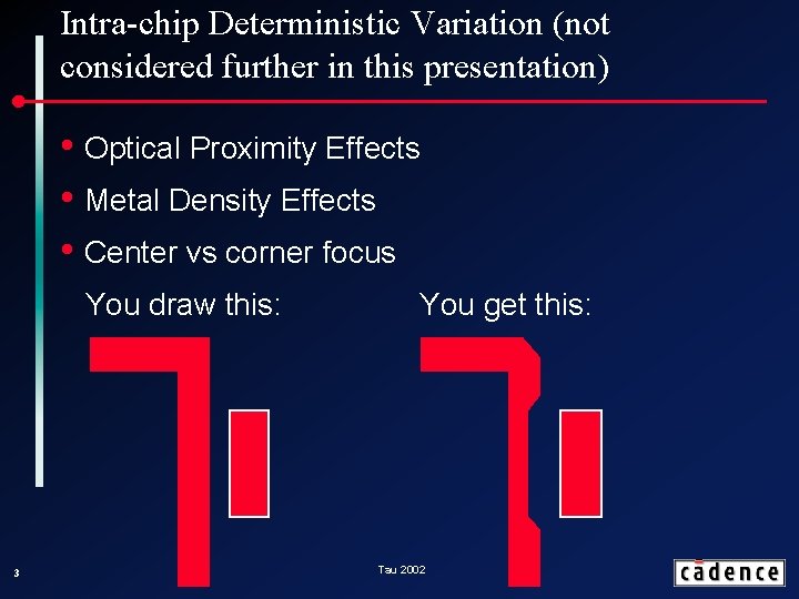
Intra-chip Deterministic Variation (not considered further in this presentation) • Optical Proximity Effects • Metal Density Effects • Center vs corner focus You draw this: 3 You get this: Tau 2002

Inter-chip variation • Many of the sources of variation affect all objects on the same layer of the same chip. • Examples: ‑ Metal or dielectric layers might be thicker/thinner ‑ Each exposure could be over/under exposed ‑ Each layer could be over/under etched 4 Tau 2002

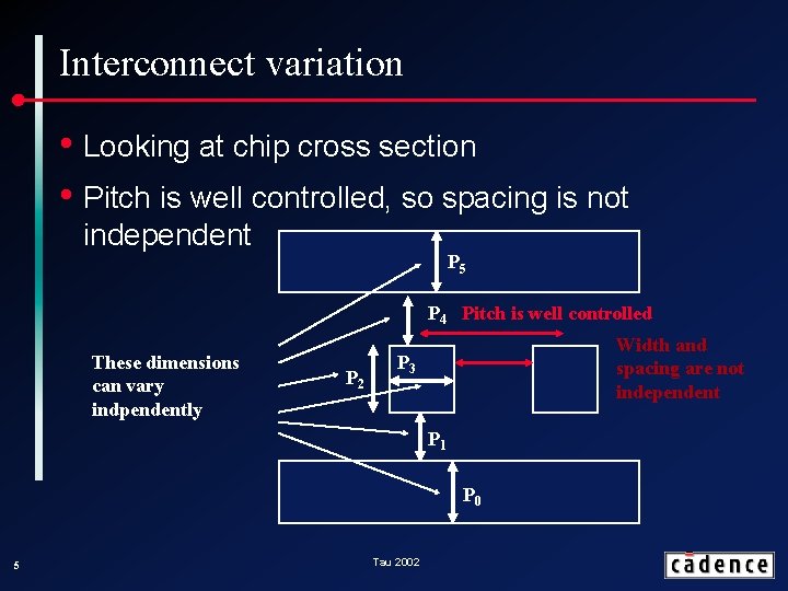
Interconnect variation • Looking at chip cross section • Pitch is well controlled, so spacing is not independent P 5 P 4 Pitch is well controlled These dimensions can vary indpendently P 2 Width and spacing are not independent P 3 P 1 P 0 5 Tau 2002

Intra-chip statistical variation • Even within a single chip, not all parameters track: ‑ Gradients ‑ Non-flat wafers ‑ Statistical variation ‣ Particularly apparent for transistors and therefore gates ‣ Small devices increase the role of variation in number of dopant atoms and DL • Analog designers have coped with this for years • Mismatch is statistical and a function of distance between two figures. 6 Tau 2002

Previous Approaches • Worst case corners – all parameters set to 3 s ‑ Does not handle intra-chip variation at all • 6 corner analysis ‑ Classify each signal/gate as clock or data ‑ Cases: both clock and data maximally slow, clock maximally slow and data almost as slow, etc. • Problems with these approaches ‑ Too pessimistic: very unlikely to get 3 s on all parameters ‑ Not pessimistic enough: doesn’t handle fast M 1, slow M 2 7 Tau 2002

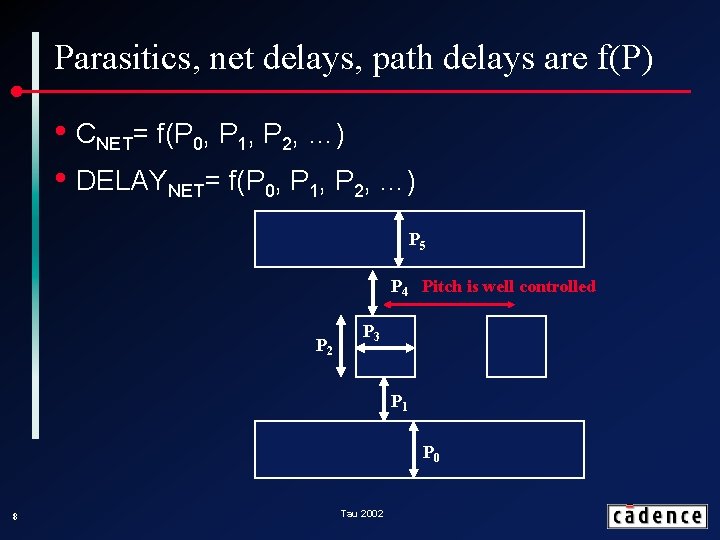
Parasitics, net delays, path delays are f(P) • CNET= f(P 0, P 1, P 2, …) • DELAYNET= f(P 0, P 1, P 2, …) P 5 P 4 Pitch is well controlled P 2 P 3 P 1 P 0 8 Tau 2002

Keeping derivatives • We represent a value as a Taylor series • Where the di describe how the value varies with a change in process parameter Dpi • Where Dpi itself has 2 parts Dpi = DGi + Dsi, d ‑ DGi is global (chip-wide variation) ‑ Dsi, d is the statistical variation of this value 9 Tau 2002

Design constraints map to fuzzy hyperplanes • The difference between data and clock must be less than the cycle time: • Which defines a fuzzy hyperplane in process space Global (Hyperplane) 10 Tau 2002 Statistical (sums to distribution)

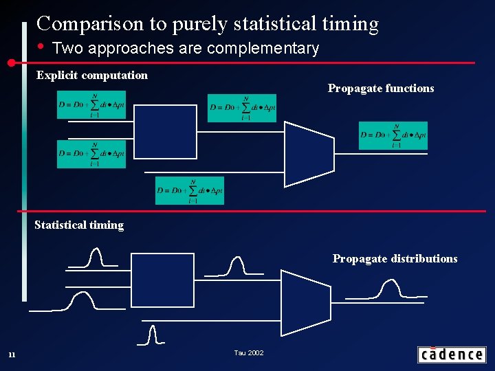
Comparison to purely statistical timing • Two approaches are complementary Explicit computation Propagate functions Statistical timing Propagate distributions 11 Tau 2002

Similarities in timing analysis • Extraction and delay reduction are straightforward, timing is not • Latest arriving signal is now poorly defined • If a significant probability for more than one signal to be last, both must be kept (or some approximate bound applied). • Pruning threshold will determine accuracy/size tradeoff. • Must compute an estimate of parametric yield at the end. • Provide a probability of failure per path for 12 optimization. Tau 2002

Differences • Propagate functions instead of distributions • Distributions of process parameters are used at different times ‑ Statistical timing needs process parameters to do timing analysis ‑ Explicit computation does timing analysis first, then plugs in process distributions to get timing distributions. ‣ Can evaluate different distributions without re-doing timing analysis 13 Tau 2002

Pruning • In statistical timing ‑ Prune if one signal is ‘almost always’ earlier ‑ Need to consider correlation because of shared input cones • ‑ Result is a distribution of delays In this explicit computation of timing ‑ Prune if one is earlier under ‘almost all’ process conditions ‑ Result is a function of process parameters ‑ Bad news – an exact answer could require (exponentially) complex functions ‑ Good news - no problem with correlation 14 Tau 2002

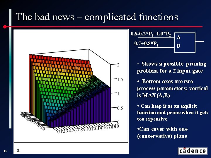
The bad news – complicated functions 0. 8 -0. 2*P 1+1. 0*P 2 0. 7+0. 5*P 1 A B • Shows a possible pruning problem for a 2 input gate • Bottom axes are two process parameters; vertical is MAX(A, B) • Can keep it as an explicit function and prune when it gets too expensive • Can cover with one (conservative) plane 15 Tau 2002

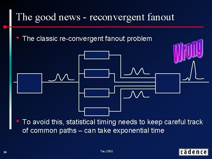
The good news - reconvergent fanout 16 • The classic re-convergent fanout problem • To avoid this, statistical timing needs to keep careful track of common paths – can take exponential time Tau 2002

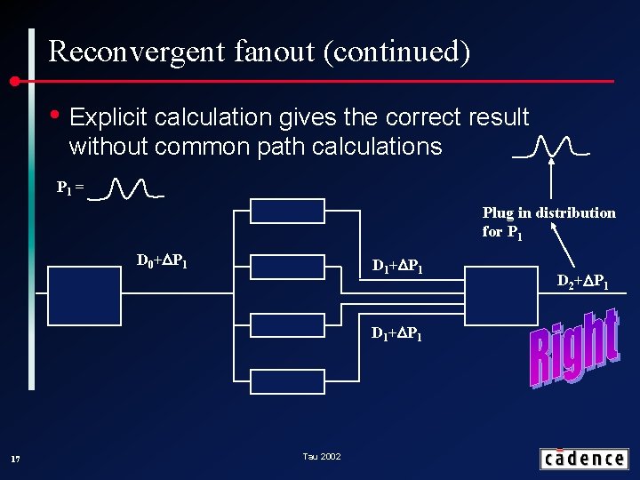
Reconvergent fanout (continued) • Explicit calculation gives the correct result without common path calculations P 1 = Plug in distribution for P 1 D 0+DP 1 D 1+DP 1 17 Tau 2002 D 2+DP 1

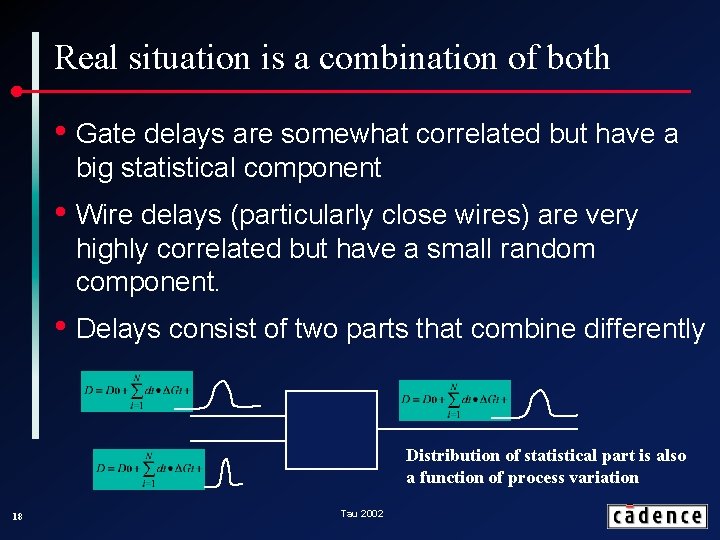
Real situation is a combination of both • Gate delays are somewhat correlated but have a big statistical component • Wire delays (particularly close wires) are very highly correlated but have a small random component. • Delays consist of two parts that combine differently Distribution of statistical part is also a function of process variation 18 Tau 2002

So what’s the point of explicit computation? • Not so worst case timing predictions ‑ Users have complained for years about timing pessimism ‑ Could be about 10% better (see experimental results) ‑ Could save months by eliminating unneeded tuning • Will catch errors that are currently missed ‑ Fast/slow combinations are not currently verified • Can predict parametric yield ‑ What’s the timing yield? ‑ How much will it help to get rid of a non-critical path? 19 Tau 2002

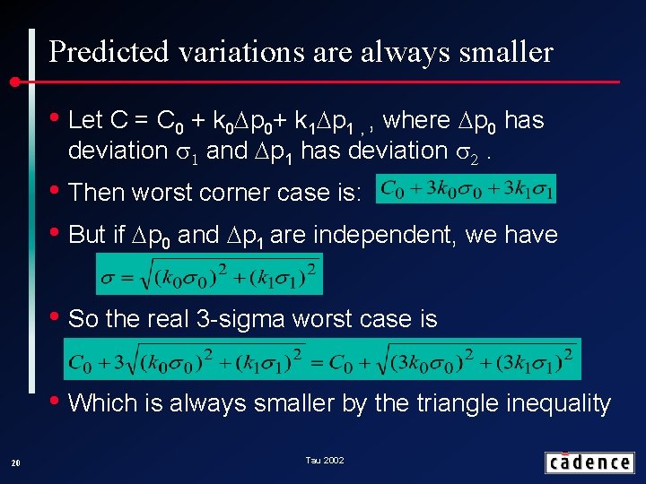
Predicted variations are always smaller • Let C = C 0 + k 0 Dp 0+ k 1 Dp 1 , , where Dp 0 has deviation s 1 and Dp 1 has deviation s 2. • Then worst corner case is: • But if Dp 0 and Dp 1 are independent, we have • So the real 3 -sigma worst case is • Which is always smaller by the triangle inequality 20 Tau 2002

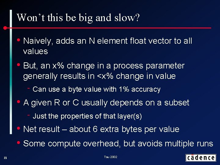
Won’t this be big and slow? • Naively, adds an N element float vector to all values • But, an x% change in a process parameter generally results in <x% change in value ‑ Can use a byte value with 1% accuracy • A given R or C usually depends on a subset ‑ Just the properties of that layer(s) • Net result – about 6 extra bytes per value • Some compute overhead, but avoids multiple runs 21 Tau 2002

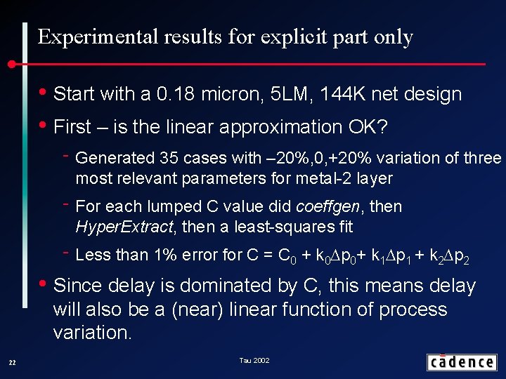
Experimental results for explicit part only • Start with a 0. 18 micron, 5 LM, 144 K net design • First – is the linear approximation OK? ‑ Generated 35 cases with – 20%, 0, +20% variation of three most relevant parameters for metal-2 layer ‑ For each lumped C value did coeffgen, then Hyper. Extract, then a least-squares fit ‑ Less than 1% error for C = C 0 + k 0 Dp 0+ k 1 Dp 1 + k 2 Dp 2 • Since delay is dominated by C, this means delay will also be a (near) linear function of process variation. 22 Tau 2002

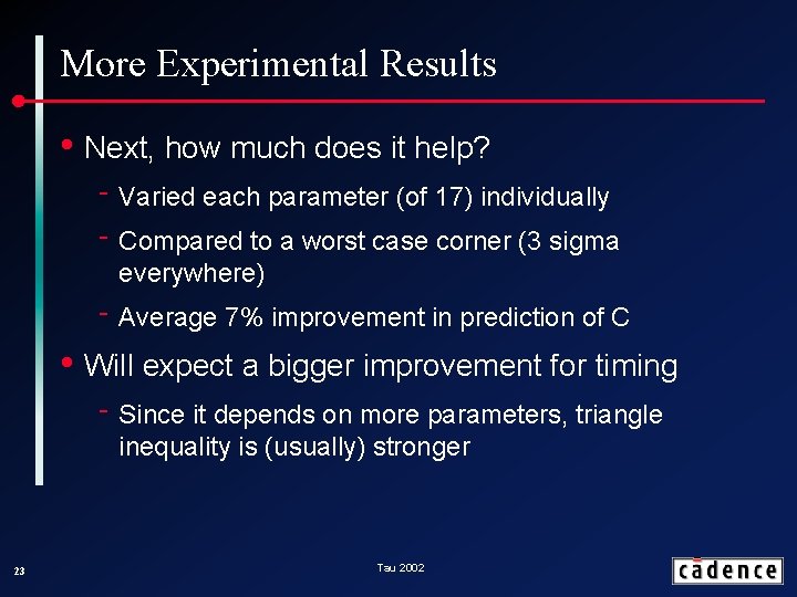
More Experimental Results • Next, how much does it help? ‑ Varied each parameter (of 17) individually ‑ Compared to a worst case corner (3 sigma everywhere) ‑ Average 7% improvement in prediction of C • Will expect a bigger improvement for timing ‑ Since it depends on more parameters, triangle inequality is (usually) stronger 23 Tau 2002

Conclusions • Outlined a possible approach for handling process variation ‑ Handles explicit and statistical variation ‑ Theory straightforward in general ‣ Pruning is the hardest part, but there are many alternatives ‑ Experiments back up assumptions needed ‑ Memory and compute time should be acceptable 24 Tau 2002