Experimental Statistics week 10 Chapter 11 Linear Regression

Experimental Statistics - week 10 Chapter 11: Linear Regression and Correlation 1

Example Probability Plots for Various Data Shapes 2

December 2000 Unemployment Rates in the 50 States 3

Distribution of Monthly Returns for all U. S. Common Stocks from 1951 - 2000 4

Distribution of Individual Salaries of Cincinnati Reds Players on Opening Day of the 2000 Season 5

Back to Correlation and Regression 6

Association Between Two Variables Correlation Analysis -- measures the strength of the linear association between 2 quantitative variables Regression Analysis -- we want to predict the dependent variable using the independent variable

Calculating the Correlation Coefficient 8

Notation: So -- 9

The data below are the study times and the test scores on an exam given over the material covered during the two weeks. Study Time (hours) Exam Score (X) (Y) 10 15 12 20 8 16 14 22 92 81 84 74 85 80 84 80 Find r 10

Population Parameter r r calculated from a set of data is an estimate of a theoretical parameter r or ryx -- in the same way the sample average is an estimate of the population mean m -- if r = 0 then there is no linear relationship between the two variables 11

Testing Statistical Significance of Correlation Coefficient Test Statistic Rejection Region t > ta/2 or t < - ta/2 df = n - 2 12

The data below are the study times and the test scores on an exam given over the material covered during the two weeks. Study Time (hours) Exam Score (X) (Y) 10 15 12 20 8 16 14 22 92 81 84 74 85 80 84 80 Test H 0: r = 0 H a: r 0 13

Correlation Between Study Time and Score Test H 0: r = 0 H a: r 0 Rejection Region: Test Statistic: Conclusion: P-value: 14

Study Time by Score The CORR Procedure 2 Variables: score Variable score time N 8 8 Mean 82. 50000 14. 62500 time Simple Statistics Std Dev Sum 5. 18239 660. 00000 4. 74906 117. 00000 Minimum 74. 00000 8. 00000 Maximum 92. 00000 22. 00000 Pearson Correlation Coefficients, N = 8 Prob > |r| under H 0: Rho=0 score time score 1. 00000 time -0. 77490 0. 0239 1. 00000 15

16

11. 1 -5 Regression Analysis 17

Notation Theoretical Model Regression line -- these are evaluated from the data 18

Data we write 19

20

Least Squares Estimates Computation Formula 21

The data below are the study times and the test scores on an exam given over the material covered during the two weeks. Study Time (hours) Exam Score (X) (Y) 10 15 12 20 8 16 14 22 92 81 84 74 85 80 84 80 Find the equation of the regression line for prediction exam score from study time. 22

Calculations: Study Time Data Equation of Regression Line: 23

PROC REG; MODEL score=time; RUN; Y X The GLM Procedure Dependent Variable: score Source Model Error Corrected Total DF 1 6 7 R-Square 0. 600470 Source time DF 1 Parameter Intercept time Sum of Squares 112. 8883610 75. 1116390 188. 0000000 Coeff Var 4. 288684 Type I SS 112. 8883610 Type III SS 112. 8883610 Estimate 94. 86698337 -0. 84560570 Mean Square 112. 8883610 12. 5186065 Root MSE 3. 538164 Pr > F 0. 0239 score Mean 82. 50000 Mean Square 112. 8883610 Standard Error 4. 30408629 0. 28159265 F Value 9. 02 t Value 22. 04 -3. 00 Pr > F 0. 0239 Pr > |t| <. 0001 0. 0239 24

To Predict Y for a given x: -- plug x into the regression equation and solve for Y Example: If a student studied 10 hours, then the predicted score would be 25

Notes: - is called the sum-of-squared residuals -- SS(Residuals) -- SSE is the estimate of the error variance 26

Testing for Significance of the Regression If knowing x is of absolutely no help in predicting Y, then it seems reasonable that the regression line for predicting Y from x should have slope ____. That is, to test for a “significant regression” we test Test Statistic Rejection Region: where t has n-2 df 27

Study Time Data 28

PROC GLM; MODEL score=time; RUN; The GLM Procedure Dependent Variable: score Source Model Error Corrected Total DF 1 6 7 Sum of Squares 112. 8883610 75. 1116390 188. 0000000 R-Square 0. 600470 Source time DF 1 Coeff Var 4. 288684 Parameter Intercept time Type I SS 112. 8883610 Type III SS 112. 8883610 Estimate 94. 86698337 -0. 84560570 Mean Square 112. 8883610 12. 5186065 Root MSE 3. 538164 Pr > F 0. 0239 score Mean 82. 50000 Mean Square 112. 8883610 Standard Error 4. 30408629 0. 28159265 F Value 9. 02 t Value 22. 04 -3. 00 Pr > F 0. 0239 Pr > |t| <. 0001 0. 0239 29

Study Time by Score The CORR Procedure 2 Variables: score Variable score time N 8 8 Mean 82. 50000 14. 62500 time Simple Statistics Std Dev Sum 5. 18239 660. 00000 4. 74906 117. 00000 Minimum 74. 00000 8. 00000 Maximum 92. 00000 22. 00000 Pearson Correlation Coefficients, N = 8 Prob > |r| under H 0: Rho=0 score time score 1. 00000 time -0. 77490 0. 0239 1. 00000 30

Note: The t values for testing H 0: r = 0 and for testing H 0: b 1 = 0 are the same. - both tests depend on the normality assumption 31

Recall: One-sample Test about a Mean df = n – 1 In general: 32

(1 – a)100% Confidence Interval for m df = n – 1 33

Similarly 34

df = n – 2 Alternative form Can also find confidence interval for b 0 - not as useful 35

Prediction Setting: 36

2 Intervals 1. Confidence Interval on m. Y|x n+1 37

38

39

2. Prediction Interval for yn+1 Notes: 40

41

Extrapolation l Predicting beyond the range of predictor variables

Predict the price of a car that weighs 3500 lbs. - extrapolation would say it’s about $16, 000 43

Predict the price of a car that weighs 3500 lbs. - extrapolation would say it’s about $16, 000 oops!!! 44

Extrapolation l • Predicting beyond the range of predictor variables NOT a good idea

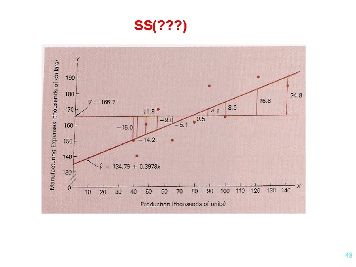
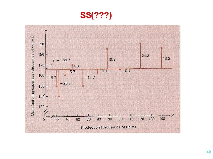
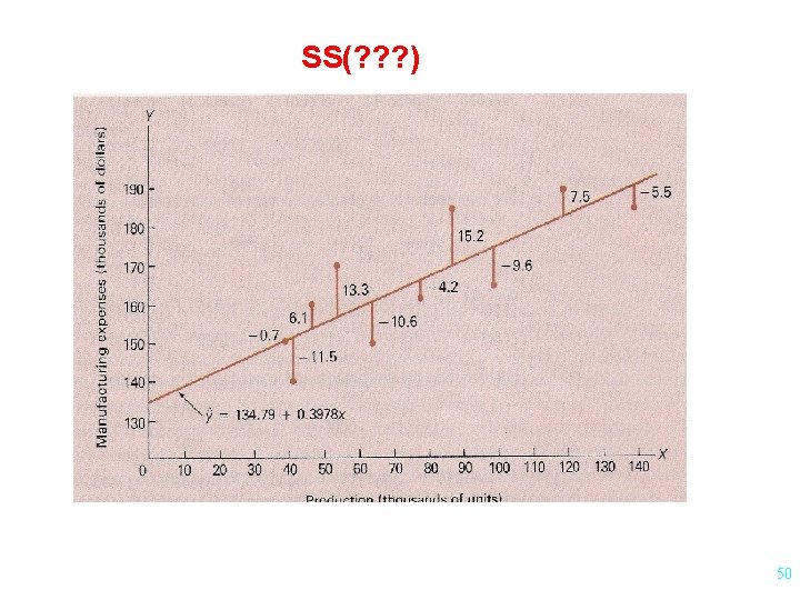
Analysis of Variance Approach Mathematical Fact SS(Total) = SS(Regression) + SS(Residuals) (Syy ) (SS “explained” by the model) (SS “unexplained” by the model) p. 649 46

Plot of Production vs Cost 47

measures the proportion of the variability in Y that is explained by the regression on X 51

Y X X 10 15 12 20 8 17 14 24 7 8 8 12 4 12 11 15 12 8 8 7 12 4 15 11 52

The REG Procedure Dependent Variable: y Source DF Model =SS(reg) 1 Error =SS(Res) 6 Corrected Total 7 =SS(Total) Sum of Squares 170. 492 23. 508 194. 000 The REG Procedure Dependent Variable: y Source DF Model 1 Error 6 Corrected Total 7 Sum of Squares 19. 575 174. 425 194. 000 53

RECALL Theoretical Model Regression line residuals 54

Residual Analysis Examination of residuals to help determine if: - assumptions are met - regression model is appropriate Residual Plot: Plot of x vs residuals 55

56

57

Study Time Data PROC REG; MODEL score=time; OUTPUT out=new r=resid; RUN; PROC GPLOT; TITLE 'Plot of Residuals'; PLOT resid*time; RUN; 58

Average Height of Girls by Age 59

Average Height of Girls by Age 60

Residual Plot 61

Residual Analysis Examination of residuals to help determine if: - assumptions are met - regression model is appropriate Residual Plot: - plot of x vs residuals Normality of Residuals: - probability plot - histogram 62