Experimental Modal Analysis 1 Shanghai Jiaotong University 2011

Experimental Modal Analysis 1 Shanghai Jiaotong University 2011

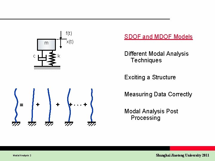
f(t) x(t) m c SDOF and MDOF Models Different Modal Analysis Techniques k Exciting a Structure Measuring Data Correctly = Modal Analysis 2 + + + + Modal Analysis Post Processing Shanghai Jiaotong University 2011

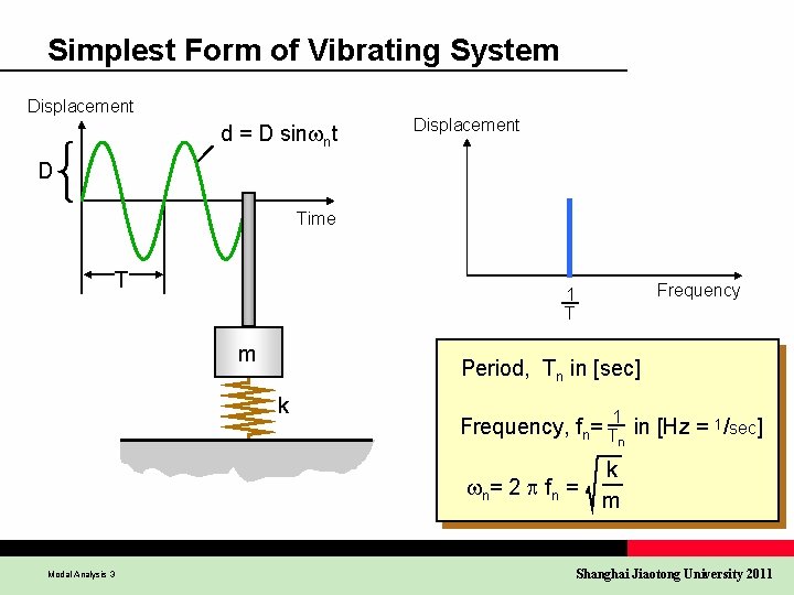
Simplest Form of Vibrating System Displacement d = D sin nt Displacement D Time T Frequency 1 T m Period, Tn in [sec] k 1 Frequency, fn= T in [Hz = 1/sec] n n = 2 f n = Modal Analysis 3 k m Shanghai Jiaotong University 2011

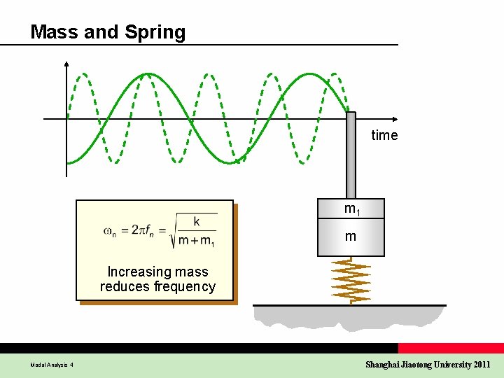
Mass and Spring time m 1 m Increasing mass reduces frequency Modal Analysis 4 Shanghai Jiaotong University 2011

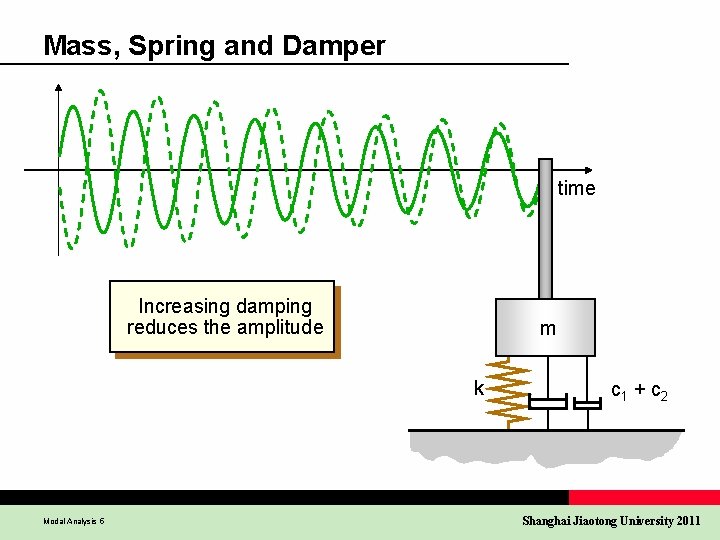
Mass, Spring and Damper time Increasing damping reduces the amplitude m k Modal Analysis 5 c 1 + c 2 Shanghai Jiaotong University 2011

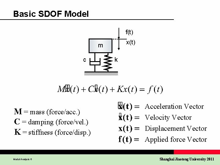
Basic SDOF Model f(t) x(t) m c M = mass (force/acc. ) C = damping (force/vel. ) K = stiffness (force/disp. ) Modal Analysis 6 k Acceleration Vector Velocity Vector Displacement Vector Applied force Vector Shanghai Jiaotong University 2011

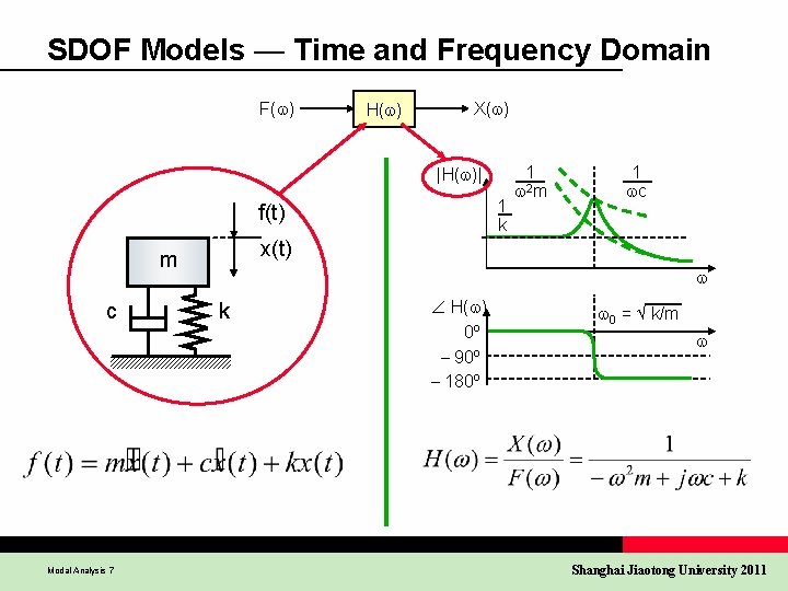
SDOF Models — Time and Frequency Domain F( ) H( ) X( ) |H( )| 1 k f(t) Modal Analysis 7 1 c x(t) m c 1 2 m k H( ) 0º – 90º – 180º 0 = k/m Shanghai Jiaotong University 2011

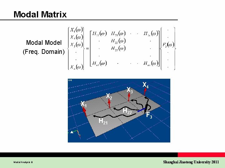
Modal Matrix Modal Model (Freq. Domain) X 1 X 2 H 21 Modal Analysis 8 X 3 X 4 F 3 Shanghai Jiaotong University 2011

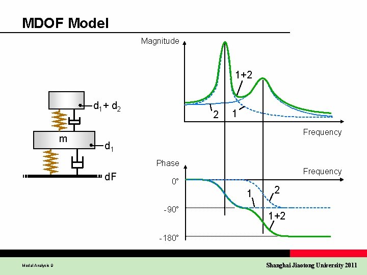
MDOF Model Magnitude 1+2 d 1 + d 2 m 2 1 Frequency d 1 Phase d. F Frequency 0° 1 -90° 2 1+2 -180° Modal Analysis 9 Shanghai Jiaotong University 2011

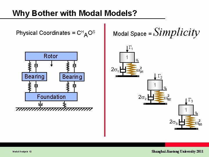
Why Bother with Modal Models? Physical Coordinates = CHAOS Modal Space = Simplicity 1 Rotor Bearing 1 q 1 2 Bearing 1 q 2 Foundation 3 1 Modal Analysis 10 q 3 Shanghai Jiaotong University 2011

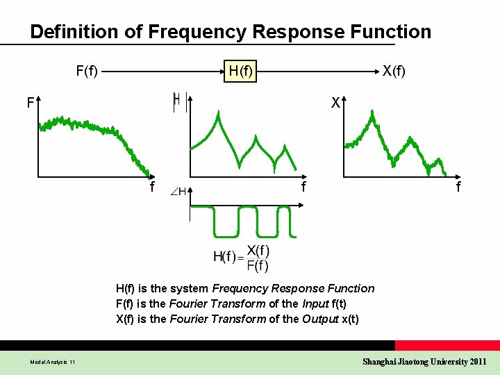
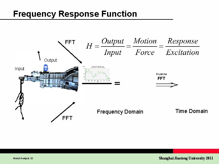
Definition of Frequency Response Function F(f) H(f) X(f) F X f f f H(f) is the system Frequency Response Function F(f) is the Fourier Transform of the Input f(t) X(f) is the Fourier Transform of the Output x(t) Modal Analysis 11 Shanghai Jiaotong University 2011

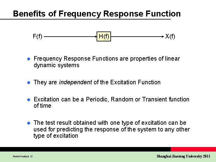
Benefits of Frequency Response Function F(f) H(f) X(f) l Frequency Response Functions are properties of linear dynamic systems l They are independent of the Excitation Function l Excitation can be a Periodic, Random or Transient function of time l The test result obtained with one type of excitation can be used for predicting the response of the system to any other type of excitation Modal Analysis 12 Shanghai Jiaotong University 2011

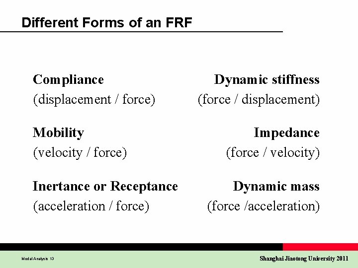
Different Forms of an FRF Compliance (displacement / force) Mobility (velocity / force) Inertance or Receptance (acceleration / force) Modal Analysis 13 Dynamic stiffness (force / displacement) Impedance (force / velocity) Dynamic mass (force /acceleration) Shanghai Jiaotong University 2011

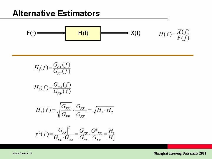
Alternative Estimators F(f) Modal Analysis 14 H(f) X(f) Shanghai Jiaotong University 2011

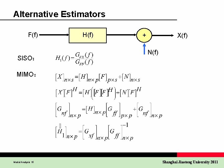
Alternative Estimators F(f) SISO： H(f) + X(f) N(f) MIMO： Modal Analysis 15 Shanghai Jiaotong University 2011

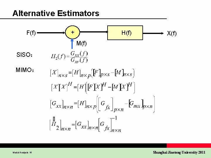
Alternative Estimators F(f) + H(f) X(f) M(f) SISO： MIMO： Modal Analysis 16 Shanghai Jiaotong University 2011

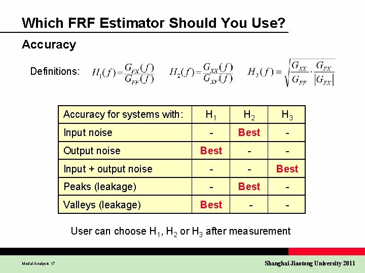
Which FRF Estimator Should You Use? Accuracy Definitions: Accuracy for systems with: H 1 H 2 H 3 - Best - - Input + output noise - - Best Peaks (leakage) - Best - Valleys (leakage) Best - - Input noise Output noise User can choose H 1, H 2 or H 3 after measurement Modal Analysis 17 Shanghai Jiaotong University 2011

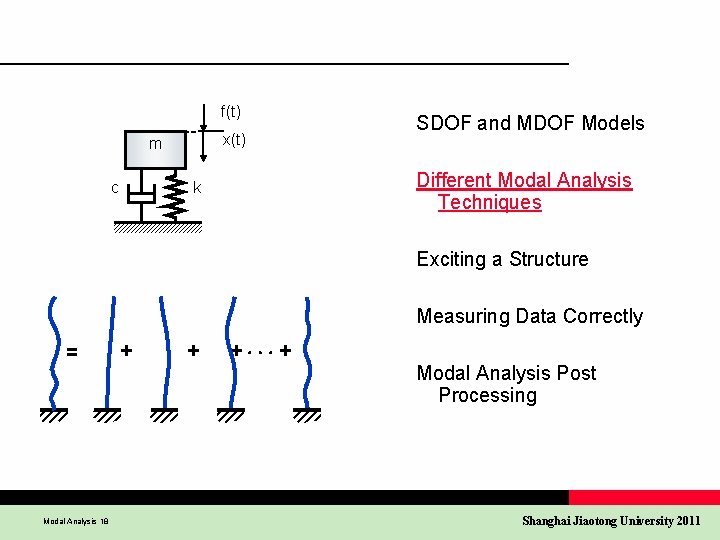
f(t) x(t) m c SDOF and MDOF Models Different Modal Analysis Techniques k Exciting a Structure Measuring Data Correctly = Modal Analysis 18 + + + + Modal Analysis Post Processing Shanghai Jiaotong University 2011

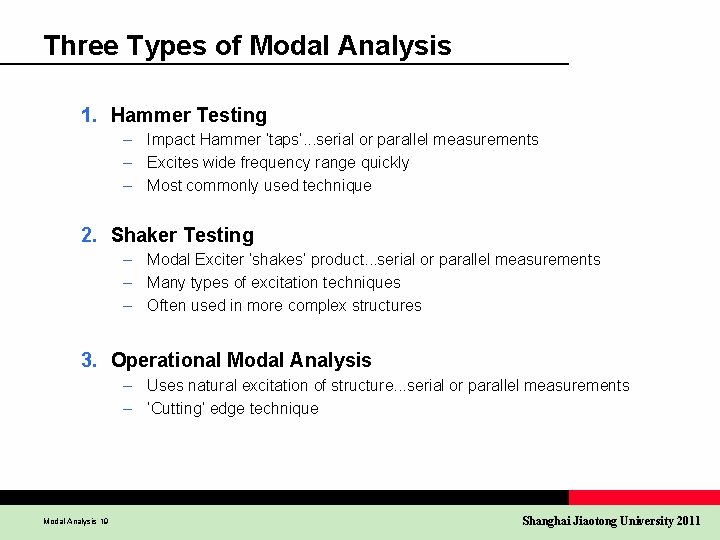
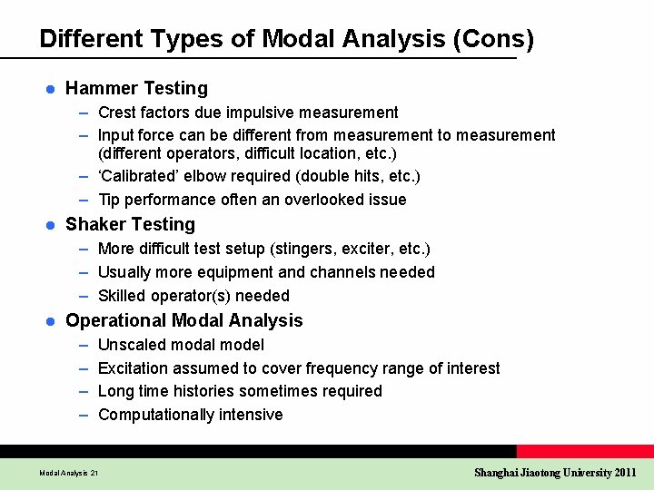
Three Types of Modal Analysis 1. Hammer Testing – Impact Hammer ’taps’. . . serial or parallel measurements – Excites wide frequency range quickly – Most commonly used technique 2. Shaker Testing – Modal Exciter ’shakes’ product. . . serial or parallel measurements – Many types of excitation techniques – Often used in more complex structures 3. Operational Modal Analysis – Uses natural excitation of structure. . . serial or parallel measurements – ’Cutting’ edge technique Modal Analysis 19 Shanghai Jiaotong University 2011

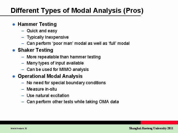
Different Types of Modal Analysis (Pros) l Hammer Testing – Quick and easy – Typically Inexpensive – Can perform ‘poor man’ modal as well as ‘full’ modal l Shaker Testing – More repeatable than hammer testing – Many types of input available – Can be used for MIMO analysis l Operational Modal Analysis – – No need for special boundary conditions Measure in-situ Use natural excitation Can perform other tests while taking OMA data Modal Analysis 20 Shanghai Jiaotong University 2011

Different Types of Modal Analysis (Cons) l Hammer Testing – Crest factors due impulsive measurement – Input force can be different from measurement to measurement (different operators, difficult location, etc. ) – ‘Calibrated’ elbow required (double hits, etc. ) – Tip performance often an overlooked issue l Shaker Testing – More difficult test setup (stingers, exciter, etc. ) – Usually more equipment and channels needed – Skilled operator(s) needed l Operational Modal Analysis – – Unscaled modal model Excitation assumed to cover frequency range of interest Long time histories sometimes required Computationally intensive Modal Analysis 21 Shanghai Jiaotong University 2011

Frequency Response Function FFT Output Inverse FFT Frequency Domain Time Domain FFT Modal Analysis 22 Shanghai Jiaotong University 2011

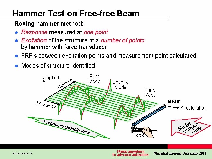
Hammer Test on Free-free Beam Roving hammer method: l Response measured at one point l Excitation of the structure at a number of points by hammer with force transducer l FRF’s between excitation points and measurement point calculated l Modes of structure identified Amplitude t Dis ce an First Mode Second Mode Third Mode Beam Acceleration Frequ ency Freq Modal Analysis 23 uenc y Do main V iew Force Force Force Press anywhere to advance animation l da ain o M om iew D V Shanghai Jiaotong University 2011

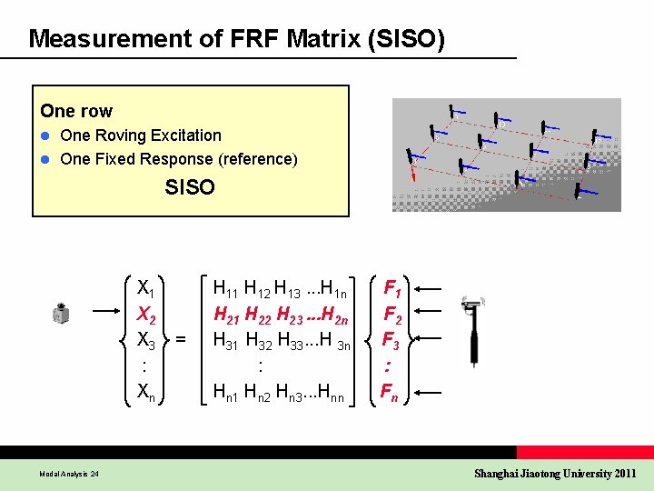
Measurement of FRF Matrix (SISO) One row One Roving Excitation l One Fixed Response (reference) l SISO X 1 X 2 X 3 : Xn Modal Analysis 24 = H 11 H 12 H 13. . . H 1 n H 21 H 22 H 23. . . H 2 n H 31 H 32 H 33. . . H 3 n : Hn 1 Hn 2 Hn 3. . . Hnn F 1 F 2 F 3 : Fn Shanghai Jiaotong University 2011

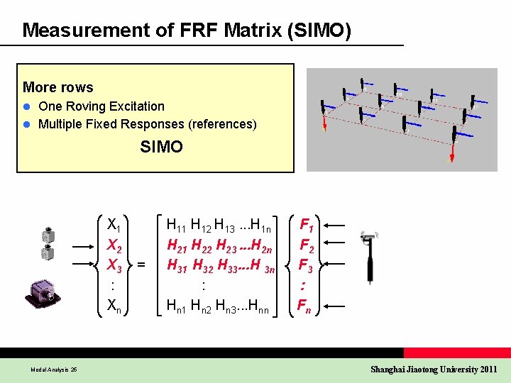
Measurement of FRF Matrix (SIMO) More rows One Roving Excitation l Multiple Fixed Responses (references) l SIMO X 1 X 2 X 3 : Xn Modal Analysis 25 = H 11 H 12 H 13. . . H 1 n H 21 H 22 H 23. . . H 2 n H 31 H 32 H 33. . . H 3 n : Hn 1 Hn 2 Hn 3. . . Hnn F 1 F 2 F 3 : Fn Shanghai Jiaotong University 2011

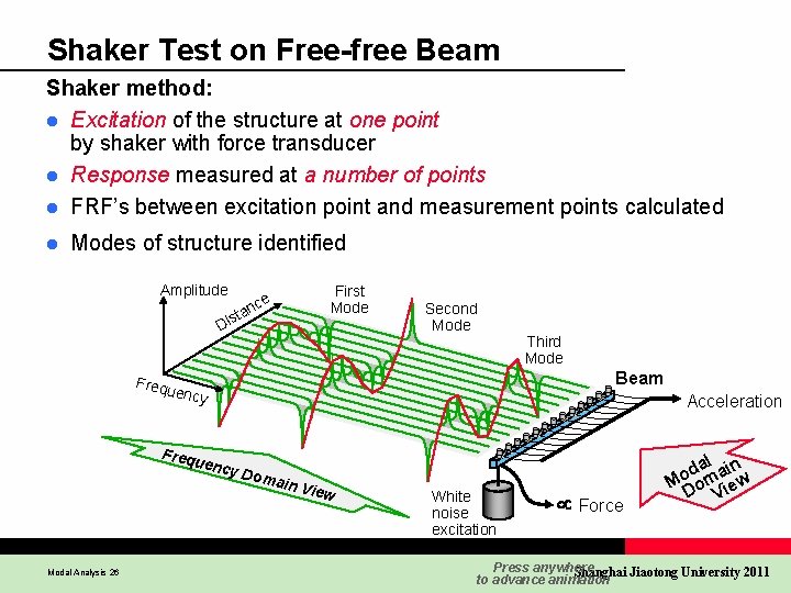
Shaker Test on Free-free Beam Shaker method: l Excitation of the structure at one point by shaker with force transducer l Response measured at a number of points l FRF’s between excitation point and measurement points calculated l Modes of structure identified Amplitude e nc a t s Di First Mode Second Mode Third Mode Beam Frequ ency Freq Modal Analysis 26 uenc y Do Acceleration main V iew White noise excitation Force l da ain o M om iew D V Press anywhere Shanghai Jiaotong University 2011 to advance animation

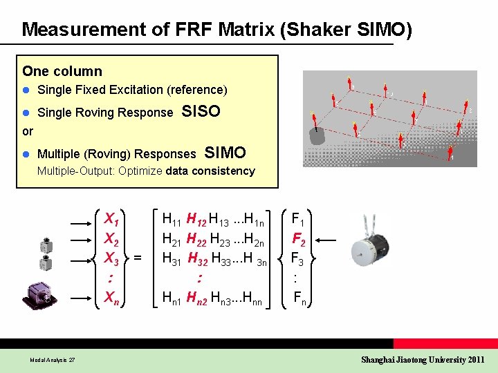
Measurement of FRF Matrix (Shaker SIMO) One column l Single Fixed Excitation (reference) l Single Roving Response SISO or l Multiple (Roving) Responses SIMO Multiple-Output: Optimize data consistency X 1 X 2 X 3 : Xn Modal Analysis 27 = H 11 H 12 H 13. . . H 1 n H 21 H 22 H 23. . . H 2 n H 31 H 32 H 33. . . H 3 n : Hn 1 Hn 2 Hn 3. . . Hnn F 1 F 2 F 3 : Fn Shanghai Jiaotong University 2011

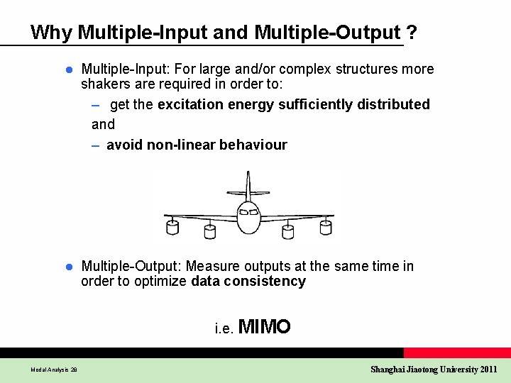
Why Multiple-Input and Multiple-Output ? l Multiple-Input: For large and/or complex structures more shakers are required in order to: – get the excitation energy sufficiently distributed and – avoid non-linear behaviour l Multiple-Output: Measure outputs at the same time in order to optimize data consistency i. e. MIMO Modal Analysis 28 Shanghai Jiaotong University 2011

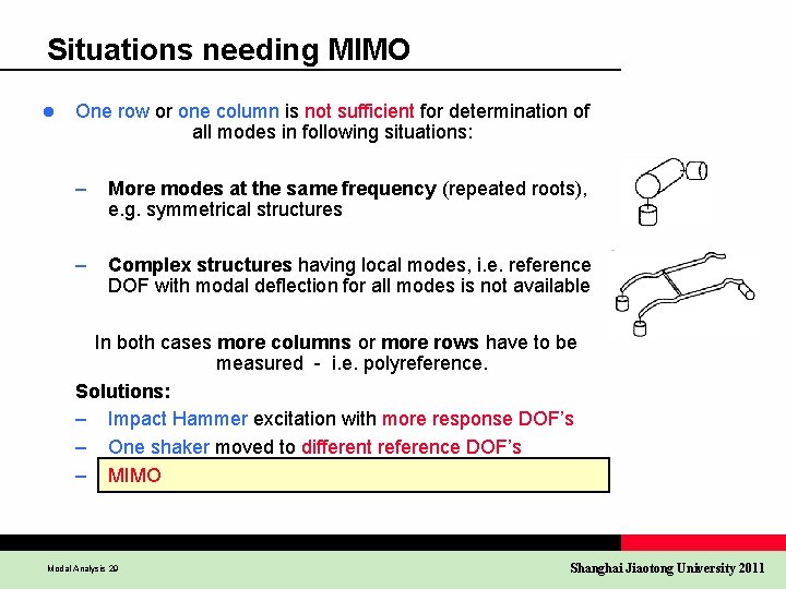
Situations needing MIMO l One row or one column is not sufficient for determination of all modes in following situations: – More modes at the same frequency (repeated roots), e. g. symmetrical structures – Complex structures having local modes, i. e. reference DOF with modal deflection for all modes is not available In both cases more columns or more rows have to be measured - i. e. polyreference. Solutions: – Impact Hammer excitation with more response DOF’s – One shaker moved to different reference DOF’s – MIMO Modal Analysis 29 Shanghai Jiaotong University 2011

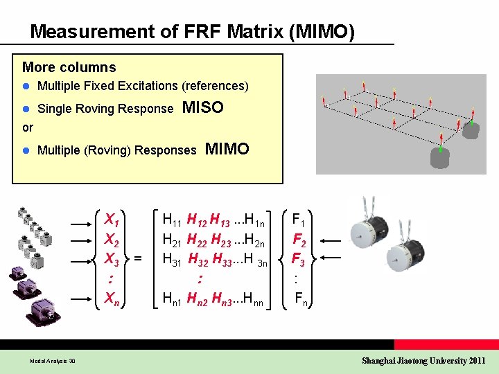
Measurement of FRF Matrix (MIMO) More columns l Multiple Fixed Excitations (references) l Single Roving Response MISO or l Multiple (Roving) Responses X 1 X 2 X 3 : Xn Modal Analysis 30 = MIMO H 11 H 12 H 13. . . H 1 n H 21 H 22 H 23. . . H 2 n H 31 H 32 H 33. . . H 3 n : Hn 1 Hn 2 Hn 3. . . Hnn F 1 F 2 F 3 : Fn Shanghai Jiaotong University 2011

Modal Analysis (classic): FRF = Response/Excitation Operational Modal Analysis (OMA): Response only! [m/s²] Time(Response) - Input Working : Input : FFT Analyzer 80 40 0 -40 -80 0 40 m 80 m 120 m [s] 160 m 200 m 240 m FFT Output Frequency Domain [m/s²] Time Domain Autospectrum(Response) - Input Working : Input : FFT Analyzer Inverse FFT 10 1 100 m Frequency Response H 1(Response, Excitation) - Input (Magnitude) [(m/s²)/N] 10 m [(m/s²)/N/s] Impulse Response h 1(Response, Excitation) - Input (Real Part) Working : Input : FFT Analyzer 2 k 1 m 10 0 200 400 600 800 [Hz] 1 k 1, 2 k 1, 4 k 1, 6 k 1 k 0 100 m Input [N] -1 k Autospectrum(Excitation) - Input Working : Input : FFT Analyzer 1 -2 k 0 100 m Natural Excitation 1 m 0 FFT Time(Excitation) - Input Working : Input : FFT Analyzer 200 100 0 -100 -200 0 40 m 80 m 120 m [s] Modal Analysis 31 160 m 200 m 240 m 400 600 800 [Hz] 1 k 1, 2 k 1, 4 k 1, 6 k 0 40 m 80 m 120 m [s] 160 m 200 m 240 m 100 u [N] 200 400 600 800 [Hz] 1 k 1, 2 k 1, 4 k 1, 6 k Frequency Response Function Impulse Response Function Response Output Vibration = H( ) = = Input Force Excitation Shanghai Jiaotong University 2011

f(t) x(t) m c SDOF and MDOF Models Different Modal Analysis Techniques k Exciting a Structure Measuring Data Correctly = Modal Analysis 32 + + + + Modal Analysis Post Processing Shanghai Jiaotong University 2011

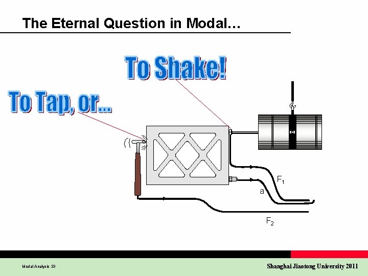
The Eternal Question in Modal… F 1 a F 2 Modal Analysis 33 Shanghai Jiaotong University 2011

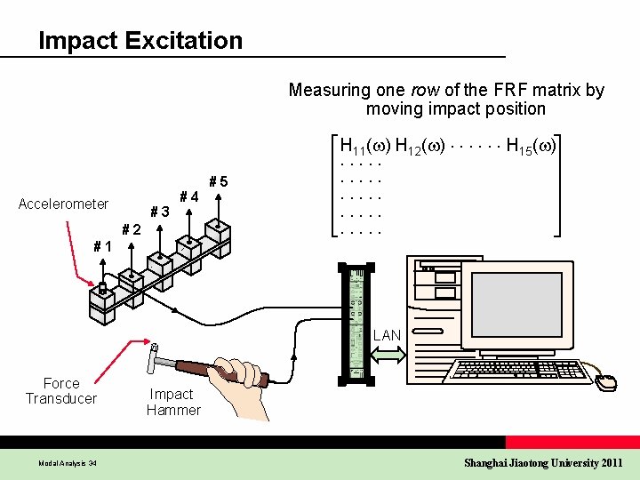
Impact Excitation Measuring one row of the FRF matrix by moving impact position Accelerometer #3 #4 #2 #1 #5 H 11( ) H 12( ) H 15( ) LAN Force Transducer Modal Analysis 34 Impact Hammer Shanghai Jiaotong University 2011

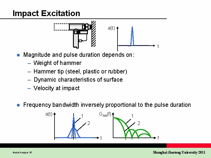
Impact Excitation a(t) t l Magnitude and pulse duration depends on: – Weight of hammer – Hammer tip (steel, plastic or rubber) – Dynamic characteristics of surface – Velocity at impact l Frequency bandwidth inversely proportional to the pulse duration a(t) GAA(f) 1 2 2 t Modal Analysis 35 1 f Shanghai Jiaotong University 2011

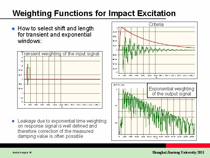
Weighting Functions for Impact Excitation l How to select shift and length for transient and exponential windows: Criteria Transient weighting of the input signal Exponential weighting of the output signal l Leakage due to exponential time weighting on response signal is well defined and therefore correction of the measured damping value is often possible Modal Analysis 36 Shanghai Jiaotong University 2011

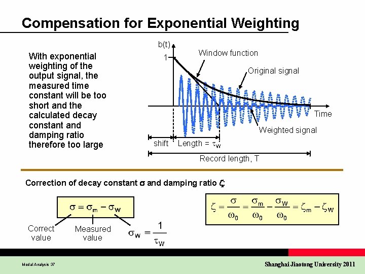
Compensation for Exponential Weighting b(t) With exponential weighting of the output signal, the measured time constant will be too short and the calculated decay constant and damping ratio therefore too large 1 Window function Original signal Time Weighted signal shift Length = Record length, T Correction of decay constant s and damping ratio z: Correct value Modal Analysis 37 Measured value Shanghai Jiaotong University 2011

Range of hammers Description Application 12 lb Sledge Building and bridges 3 lb Hand Sledge Large shafts and larger machine tools Car framed and machine tools 1 lb hammer Modal Analysis 38 General Purpose, 0. 3 lb Components Mini Hammer Hard-drives, circuit boards, turbine blades Shanghai Jiaotong University 2011

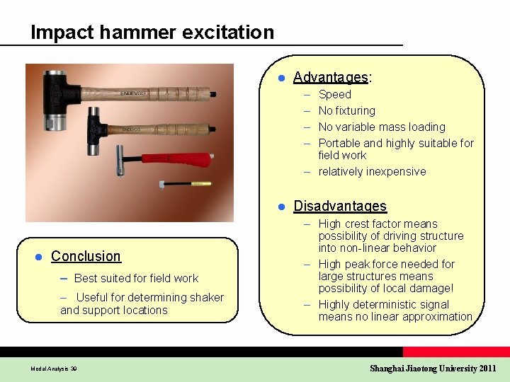
Impact hammer excitation l Advantages: – – Speed No fixturing No variable mass loading Portable and highly suitable for field work – relatively inexpensive l l Conclusion – Best suited for field work – Useful for determining shaker and support locations Modal Analysis 39 Disadvantages – High crest factor means possibility of driving structure into non-linear behavior – High peak force needed for large structures means possibility of local damage! – Highly deterministic signal means no linear approximation Shanghai Jiaotong University 2011

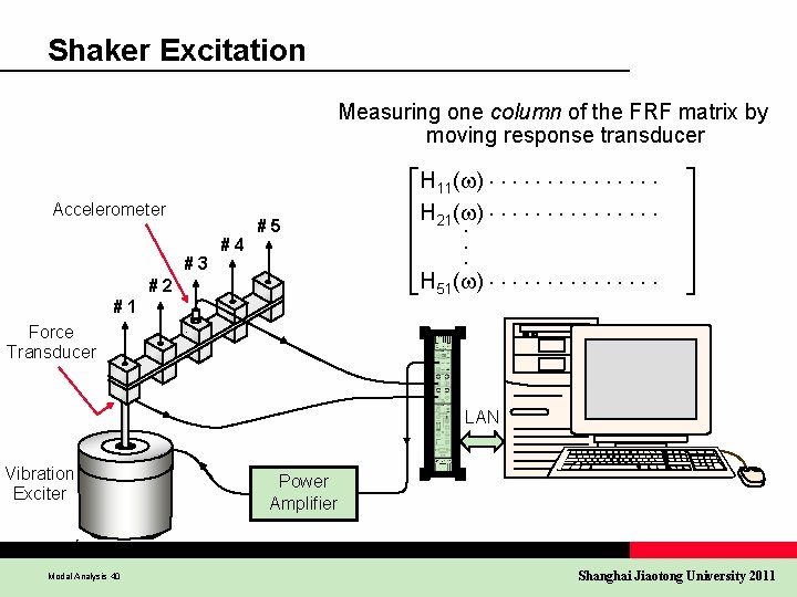
Shaker Excitation Measuring one column of the FRF matrix by moving response transducer Accelerometer #3 #4 #5 #2 #1 H 11( ) H 21( ) H 51( ) Force Transducer LAN Vibration Exciter Modal Analysis 40 Power Amplifier Shanghai Jiaotong University 2011

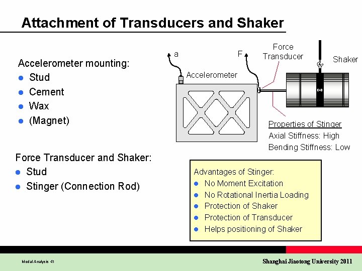
Attachment of Transducers and Shaker Accelerometer mounting: l Stud l Cement l Wax l (Magnet) Force Transducer and Shaker: l Stud l Stinger (Connection Rod) Modal Analysis 41 a F Force Transducer Shaker Accelerometer Properties of Stinger Axial Stiffness: High Bending Stiffness: Low Advantages of Stinger: l No Moment Excitation l No Rotational Inertia Loading l Protection of Shaker l Protection of Transducer l Helps positioning of Shaker Shanghai Jiaotong University 2011

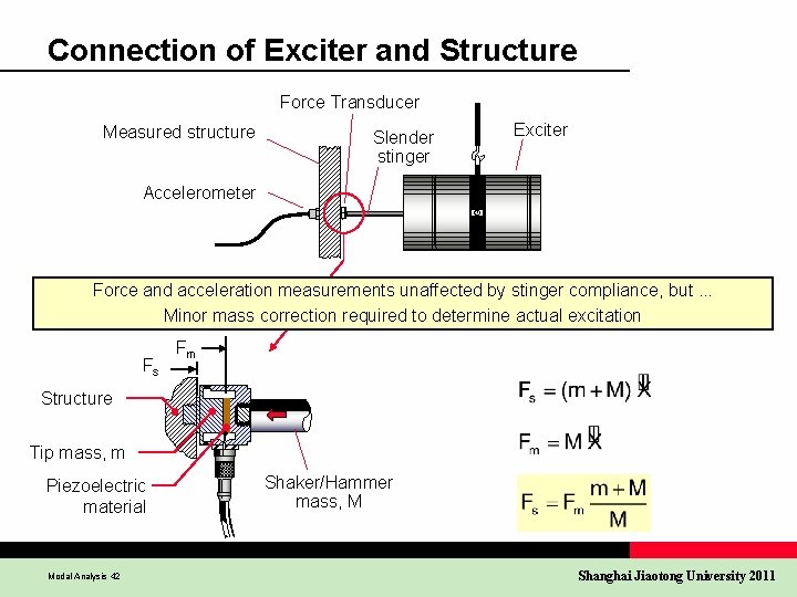
Connection of Exciter and Structure Force Transducer Measured structure Slender stinger Exciter Accelerometer Force and acceleration measurements unaffected by stinger compliance, but. . . Minor mass correction required to determine actual excitation Fs Fm Structure Tip mass, m Piezoelectric material Modal Analysis 42 Shaker/Hammer mass, M Shanghai Jiaotong University 2011

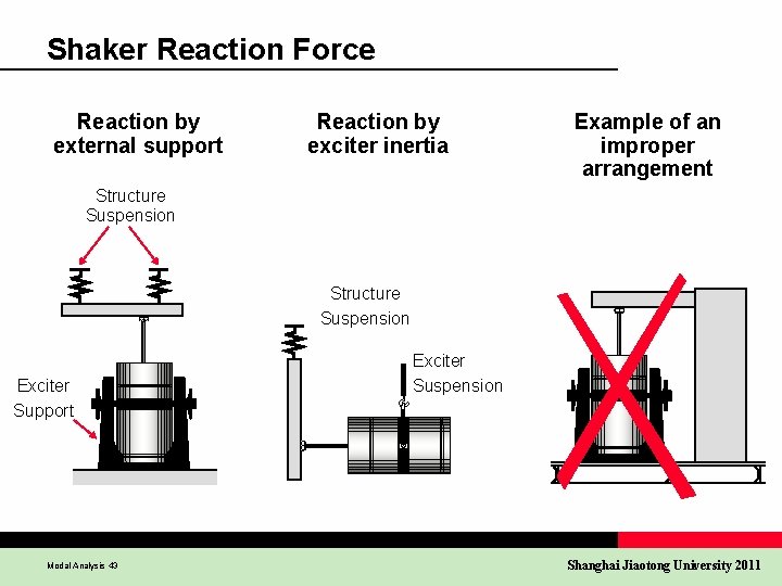
Shaker Reaction Force Reaction by external support Reaction by exciter inertia Example of an improper arrangement Structure Suspension Exciter Support Modal Analysis 43 Exciter Suspension Shanghai Jiaotong University 2011

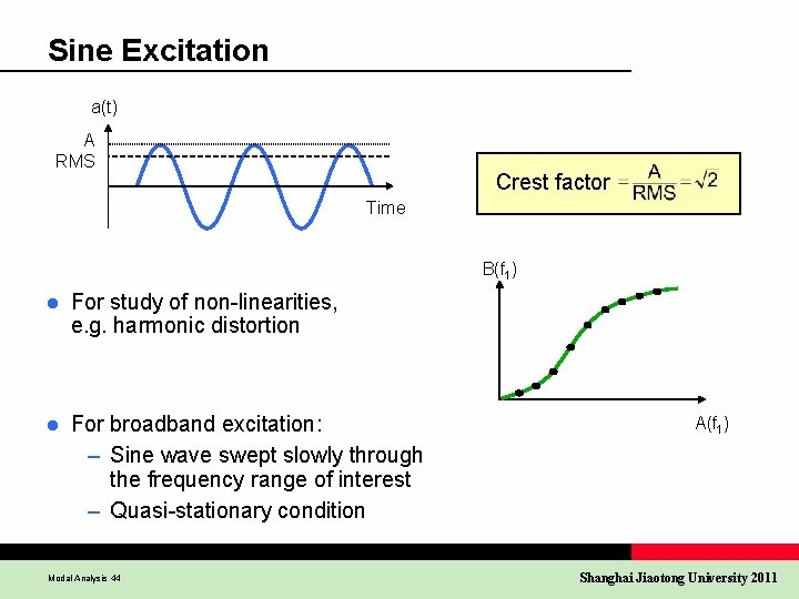
Sine Excitation a(t) A RMS Crest factor Time B(f 1) l For study of non-linearities, e. g. harmonic distortion l For broadband excitation: – Sine wave swept slowly through the frequency range of interest – Quasi-stationary condition Modal Analysis 44 A(f 1) Shanghai Jiaotong University 2011

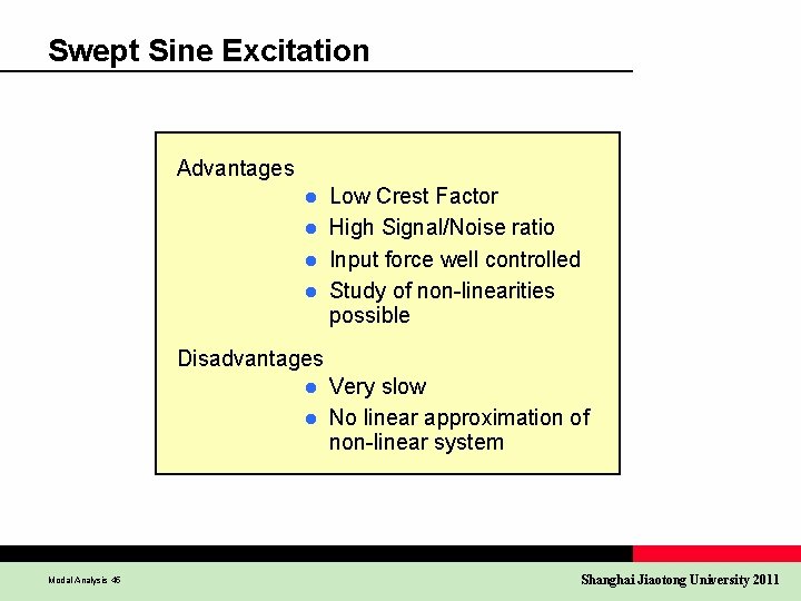
Swept Sine Excitation Advantages Low Crest Factor l High Signal/Noise ratio l Input force well controlled l Study of non-linearities possible l Disadvantages Very slow l No linear approximation of non-linear system l Modal Analysis 45 Shanghai Jiaotong University 2011

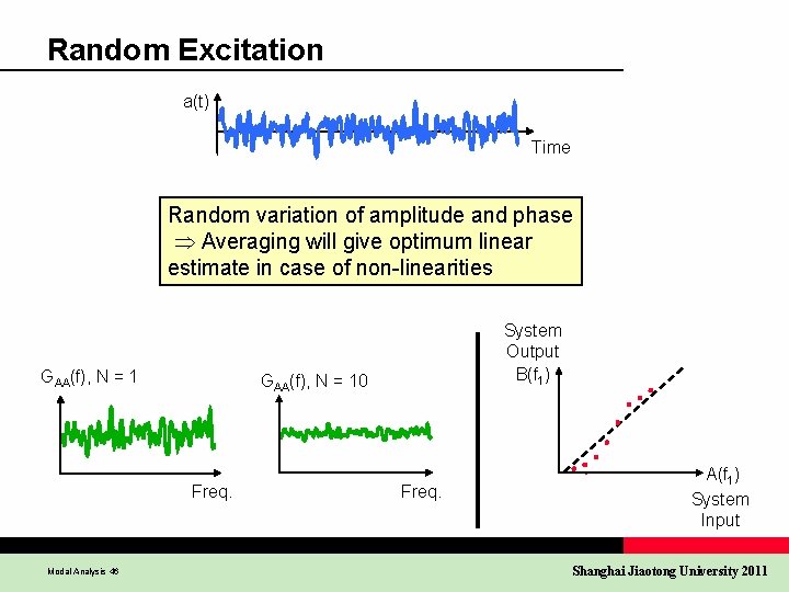
Random Excitation a(t) Time Random variation of amplitude and phase Averaging will give optimum linear estimate in case of non-linearities GAA(f), N = 10 Freq. Modal Analysis 46 System Output B(f 1) Freq. A(f 1) System Input Shanghai Jiaotong University 2011

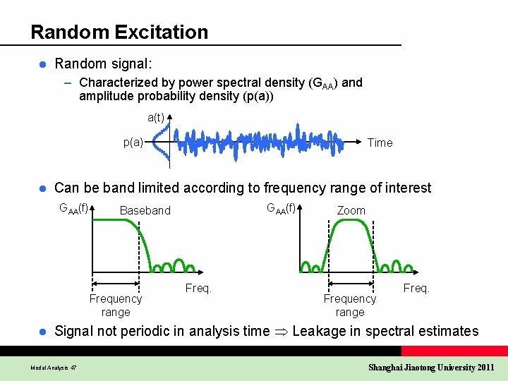
Random Excitation l Random signal: – Characterized by power spectral density (GAA) and amplitude probability density (p(a)) a(t) p(a) l Can be band limited according to frequency range of interest GAA(f) Baseband Frequency range l Time Freq. Zoom Frequency range Freq. Signal not periodic in analysis time Leakage in spectral estimates Modal Analysis 47 Shanghai Jiaotong University 2011

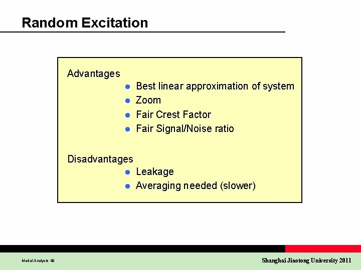
Random Excitation Advantages Best linear approximation of system l Zoom l Fair Crest Factor l Fair Signal/Noise ratio l Disadvantages Leakage l Averaging needed (slower) l Modal Analysis 48 Shanghai Jiaotong University 2011

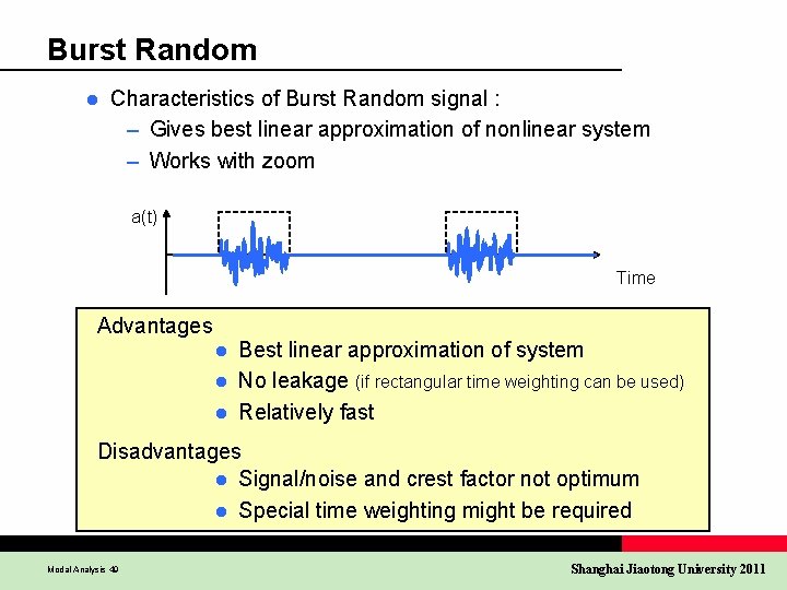
Burst Random l Characteristics of Burst Random signal : – Gives best linear approximation of nonlinear system – Works with zoom a(t) Time Advantages Best linear approximation of system l No leakage (if rectangular time weighting can be used) l Relatively fast l Disadvantages l Signal/noise and crest factor not optimum l Special time weighting might be required Modal Analysis 49 Shanghai Jiaotong University 2011

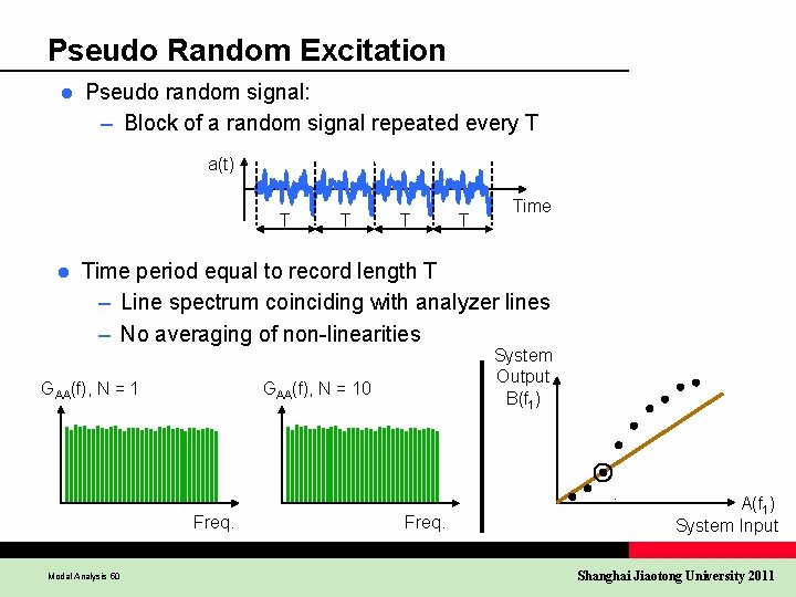
Pseudo Random Excitation l Pseudo random signal: – Block of a random signal repeated every T a(t) T l T Time period equal to record length T – Line spectrum coinciding with analyzer lines – No averaging of non-linearities GAA(f), N = 10 Freq. Modal Analysis 50 System Output B(f 1) Freq. A(f 1) System Input Shanghai Jiaotong University 2011

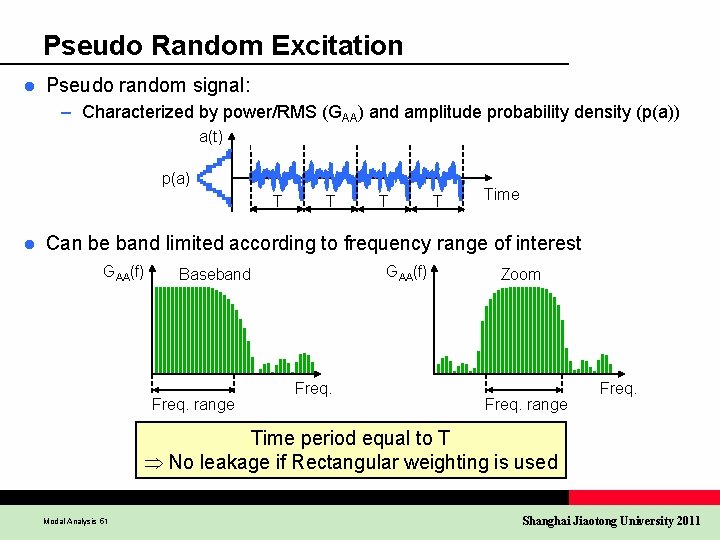
Pseudo Random Excitation l Pseudo random signal: – Characterized by power/RMS (GAA) and amplitude probability density (p(a)) a(t) p(a) T l T Time Can be band limited according to frequency range of interest GAA(f) Baseband Freq. range Freq. Zoom Freq. range Freq. Time period equal to T No leakage if Rectangular weighting is used Modal Analysis 51 Shanghai Jiaotong University 2011

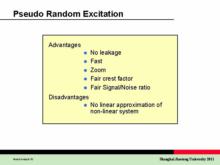
Pseudo Random Excitation Advantages l l l No leakage Fast Zoom Fair crest factor Fair Signal/Noise ratio Disadvantages l Modal Analysis 52 No linear approximation of non-linear system Shanghai Jiaotong University 2011

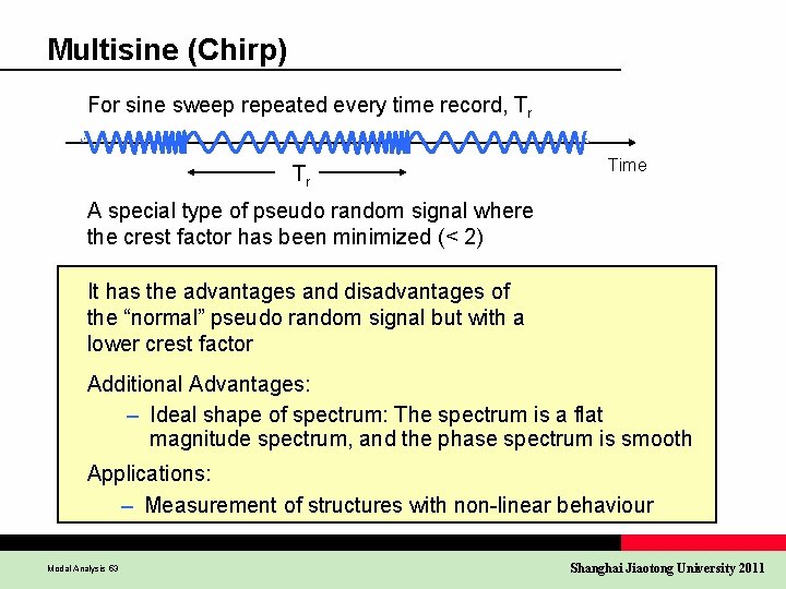
Multisine (Chirp) For sine sweep repeated every time record, Tr Tr Time A special type of pseudo random signal where the crest factor has been minimized (< 2) It has the advantages and disadvantages of the “normal” pseudo random signal but with a lower crest factor Additional Advantages: – Ideal shape of spectrum: The spectrum is a flat magnitude spectrum, and the phase spectrum is smooth Applications: – Measurement of structures with non-linear behaviour Modal Analysis 53 Shanghai Jiaotong University 2011

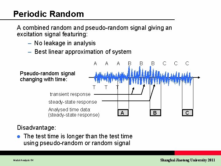
Periodic Random A combined random and pseudo-random signal giving an excitation signal featuring: – No leakage in analysis – Best linear approximation of system A A A T T T B B B C C C Pseudo-random signal changing with time: transient response steady-state response Analysed time data: (steady-state response) A B C Disadvantage: l The test time is longer than the test time using pseudo-random or random signal Modal Analysis 54 Shanghai Jiaotong University 2011

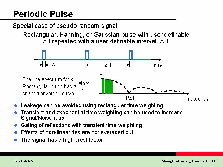
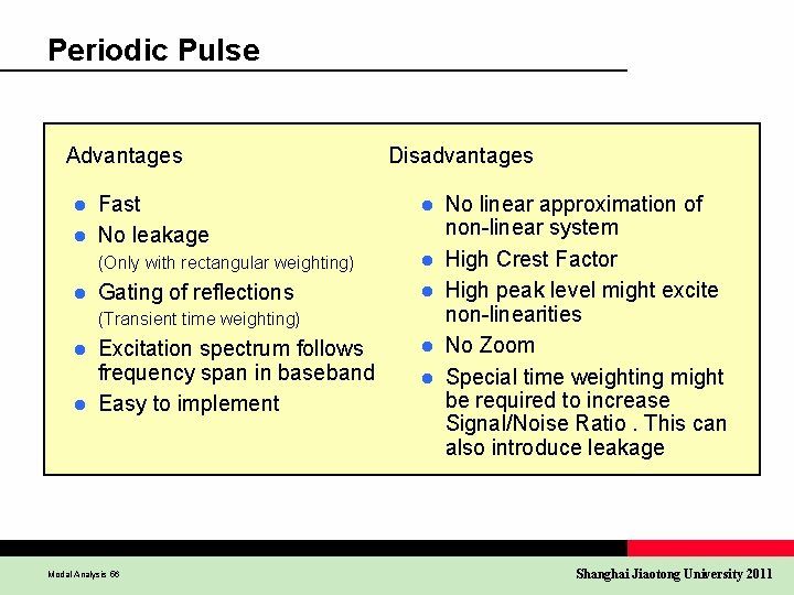
Periodic Pulse Special case of pseudo random signal Rectangular, Hanning, or Gaussian pulse with user definable D t repeated with a user definable interval, D T Dt The line spectrum for a sin x Rectangular pulse has a x shaped envelope curve l l l DT Time 1/D t Frequency Leakage can be avoided using rectangular time weighting Transient and exponential time weighting can be used to increase Signal/Noise ratio Gating of reflections with transient time weighting Effects of non-linearities are not averaged out The signal has a high crest factor Modal Analysis 55 Shanghai Jiaotong University 2011

Periodic Pulse Advantages Fast l No leakage l l Disadvantages l (Only with rectangular weighting) l Gating of reflections l (Transient time weighting) Excitation spectrum follows frequency span in baseband l Easy to implement l Modal Analysis 56 l l No linear approximation of non-linear system High Crest Factor High peak level might excite non-linearities No Zoom Special time weighting might be required to increase Signal/Noise Ratio. This can also introduce leakage Shanghai Jiaotong University 2011

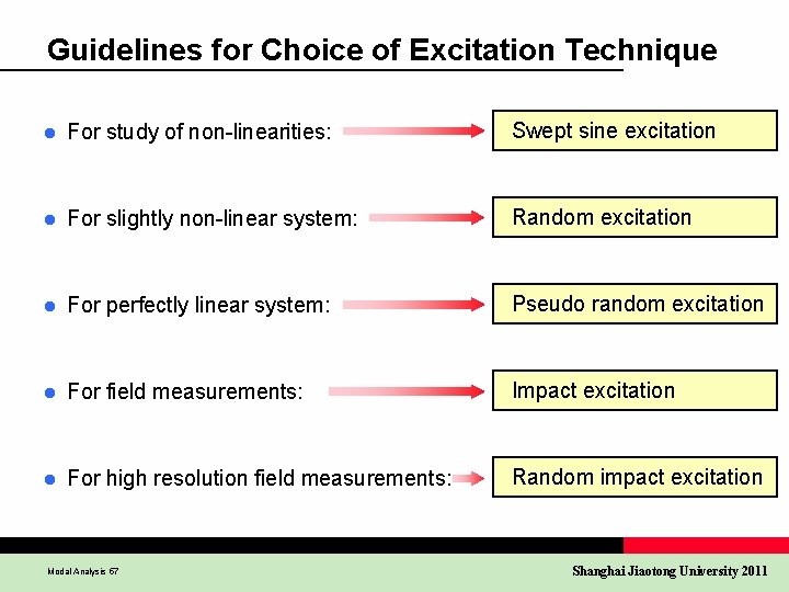
Guidelines for Choice of Excitation Technique l For study of non-linearities: Swept sine excitation l For slightly non-linear system: Random excitation l For perfectly linear system: Pseudo random excitation l For field measurements: Impact excitation l For high resolution field measurements: Random impact excitation Modal Analysis 57 Shanghai Jiaotong University 2011

f(t) x(t) m c SDOF and MDOF Models Different Modal Analysis Techniques k Exciting a Structure Measuring Data Correctly = Modal Analysis 58 + + + + Modal Analysis Post Processing Shanghai Jiaotong University 2011

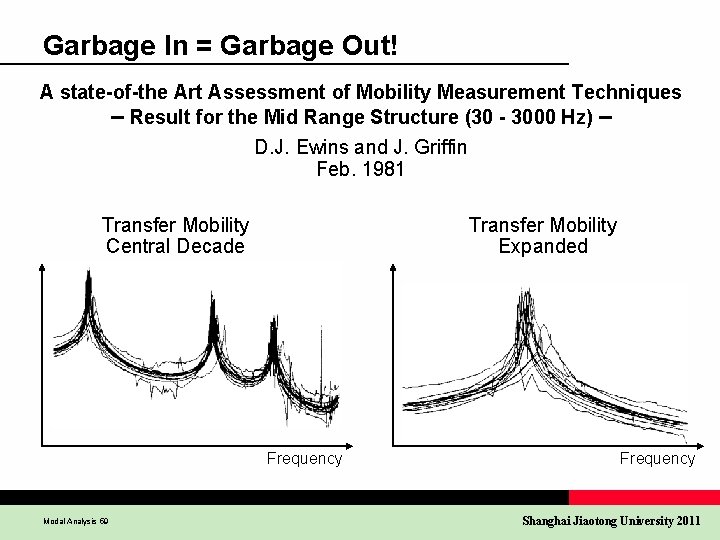
Garbage In = Garbage Out! A state-of-the Art Assessment of Mobility Measurement Techniques – Result for the Mid Range Structure (30 - 3000 Hz) – D. J. Ewins and J. Griffin Feb. 1981 Transfer Mobility Central Decade Transfer Mobility Expanded Frequency Modal Analysis 59 Frequency Shanghai Jiaotong University 2011

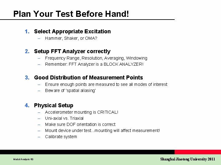
Plan Your Test Before Hand! 1. Select Appropriate Excitation – Hammer, Shaker, or OMA? 2. Setup FFT Analyzer correctly – – Frequency Range, Resolution, Averaging, Windowing Remember: FFT Analyzer is a BLOCK ANALYZER! 3. Good Distribution of Measurement Points – – Ensure enough points are measured to see all modes of interest Beware of ’spatial aliasing’ 4. Physical Setup – – – Modal Analysis 60 Accelerometer mounting is CRITICAL! Uni-axial vs. Triaxial Make sure DOF orientation is correct Mount device under test. . . mounting will affect measurement! Calibrate system Shanghai Jiaotong University 2011

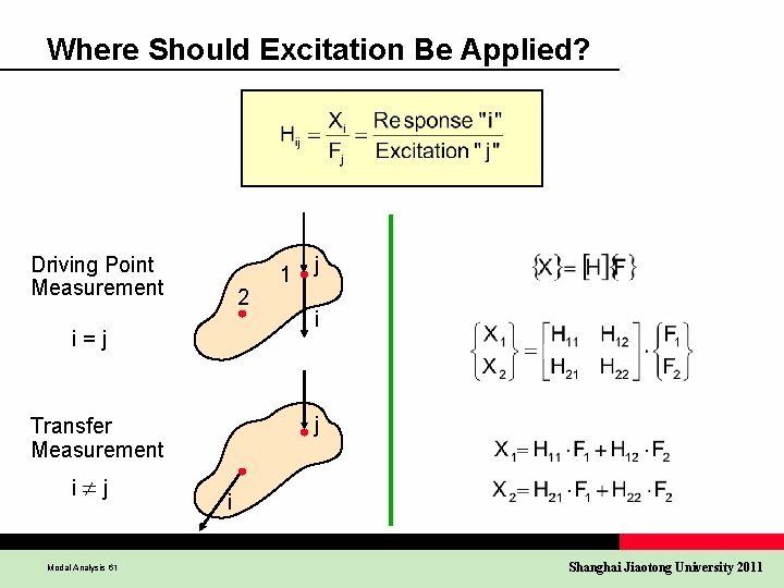
Where Should Excitation Be Applied? Driving Point Measurement 2 i=j Modal Analysis 61 j i j Transfer Measurement i¹j 1 i Shanghai Jiaotong University 2011

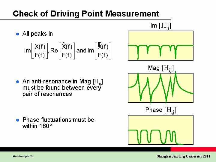
Check of Driving Point Measurement l All peaks in Im Hij Mag Hij l An anti-resonance in Mag Hij must be found between every pair of resonances Phase Hij l Phase fluctuations must be within 180 Modal Analysis 62 Shanghai Jiaotong University 2011

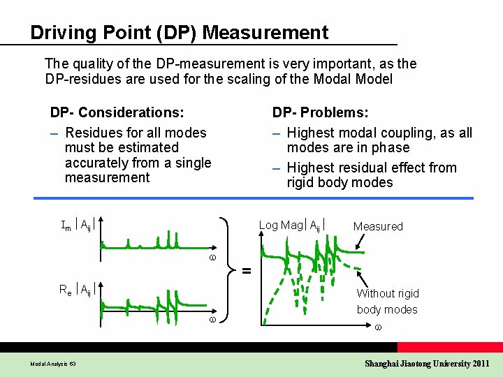
Driving Point (DP) Measurement The quality of the DP-measurement is very important, as the DP-residues are used for the scaling of the Modal Model DP- Considerations: – Residues for all modes must be estimated accurately from a single measurement DP- Problems: – Highest modal coupling, as all modes are in phase – Highest residual effect from rigid body modes m Aij Log Mag Aij Re Aij Modal Analysis 63 Measured = Without rigid body modes Shanghai Jiaotong University 2011

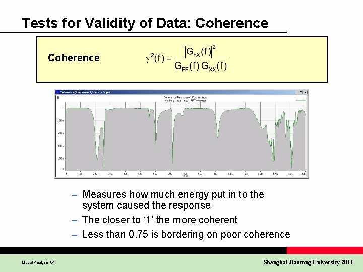
Tests for Validity of Data: Coherence – Measures how much energy put in to the system caused the response – The closer to ‘ 1’ the more coherent – Less than 0. 75 is bordering on poor coherence Modal Analysis 64 Shanghai Jiaotong University 2011

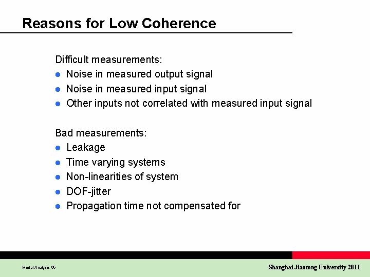
Reasons for Low Coherence Difficult measurements: l Noise in measured output signal l Noise in measured input signal l Other inputs not correlated with measured input signal Bad measurements: l Leakage l Time varying systems l Non-linearities of system l DOF-jitter l Propagation time not compensated for Modal Analysis 65 Shanghai Jiaotong University 2011

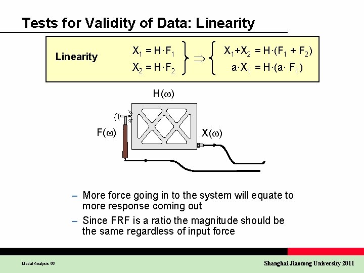
Tests for Validity of Data: Linearity X 1 = H·F 1 X 2 = H·F 2 X 1+X 2 = H·(F 1 + F 2) a·X 1 = H·(a· F 1) H( ) F( ) X( ) – More force going in to the system will equate to more response coming out – Since FRF is a ratio the magnitude should be the same regardless of input force Modal Analysis 66 Shanghai Jiaotong University 2011

Tips and Tricks for Best Results l Verify measurement chain integrity prior to test: – Transducer calibration – Mass Ratio calibration l Verify suitability of input and output transducers: – – – l Operating ranges (frequency, dynamic range, phase response) Mass loading of accelerometers Accelerometer mounting Sensitivity to environmental effects Stability Verify suitability of test set-up: – Transducer positioning and alignment – Pre-test: rattling, boundary conditions, rigid body modes, signal-to-noise ratio, linear approximation, excitation signal, repeated roots, Maxwell reciprocity, force measurement, exciter-input transducer-stinger-structure connection Quality FRF measurements are the foundation of experimental modal analysis! Modal Analysis 67 Shanghai Jiaotong University 2011

f(t) x(t) m c SDOF and MDOF Models Different Modal Analysis Techniques k Exciting a Structure Measuring Data Correctly = Modal Analysis 68 + + + + Modal Analysis Post Processing Shanghai Jiaotong University 2011

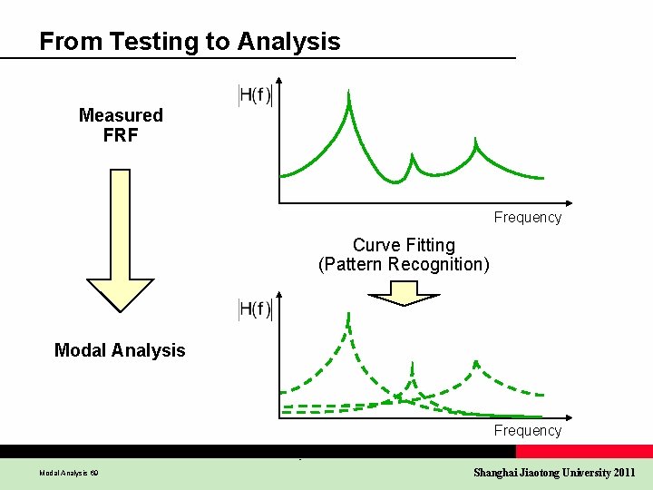
From Testing to Analysis Measured FRF Frequency Curve Fitting (Pattern Recognition) Modal Analysis Frequency Modal Analysis 69 Shanghai Jiaotong University 2011

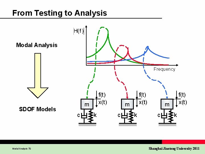
From Testing to Analysis Modal Analysis Frequency SDOF Models Modal Analysis 70 f(t) x(t) m c k Shanghai Jiaotong University 2011

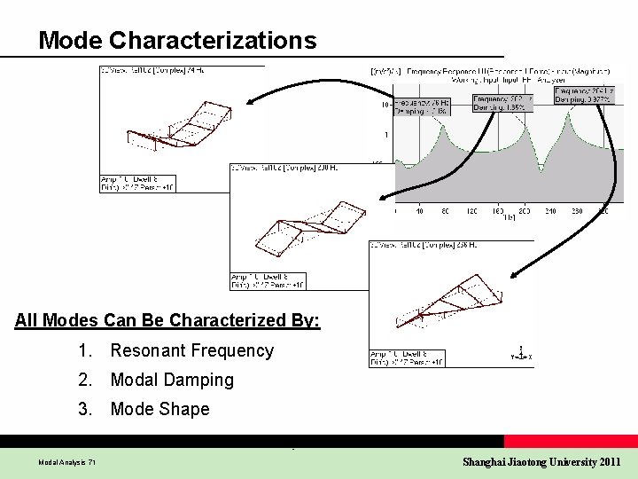
Mode Characterizations All Modes Can Be Characterized By: 1. Resonant Frequency 2. Modal Damping 3. Mode Shape Modal Analysis 71 Shanghai Jiaotong University 2011

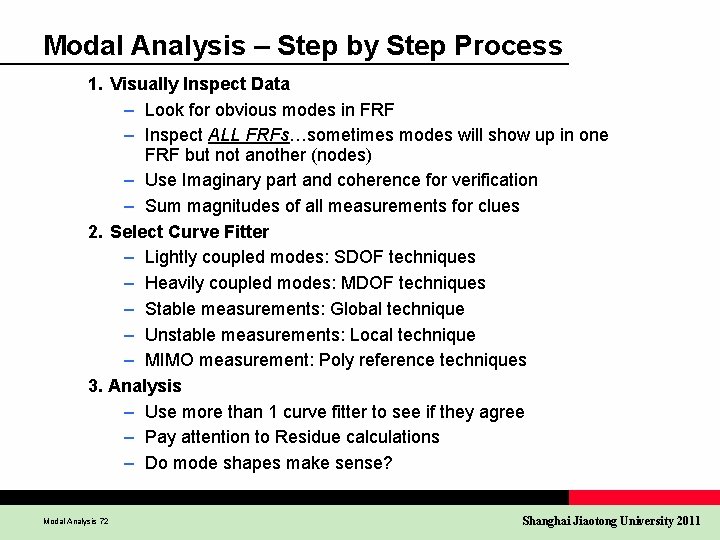
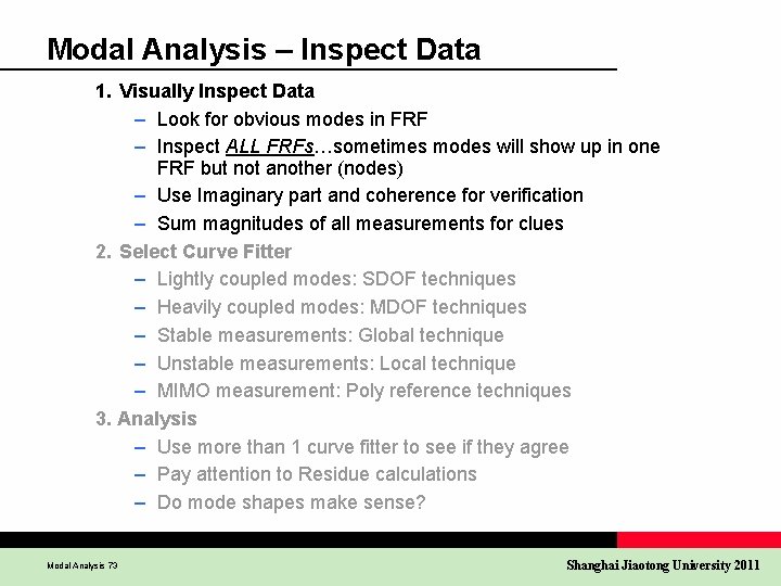
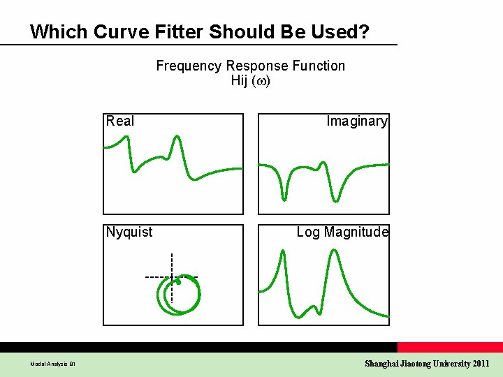
Modal Analysis – Step by Step Process 1. Visually Inspect Data – Look for obvious modes in FRF – Inspect ALL FRFs…sometimes modes will show up in one FRF but not another (nodes) – Use Imaginary part and coherence for verification – Sum magnitudes of all measurements for clues 2. Select Curve Fitter – Lightly coupled modes: SDOF techniques – Heavily coupled modes: MDOF techniques – Stable measurements: Global technique – Unstable measurements: Local technique – MIMO measurement: Poly reference techniques 3. Analysis – Use more than 1 curve fitter to see if they agree – Pay attention to Residue calculations – Do mode shapes make sense? Modal Analysis 72 Shanghai Jiaotong University 2011

Modal Analysis – Inspect Data 1. Visually Inspect Data – Look for obvious modes in FRF – Inspect ALL FRFs…sometimes modes will show up in one FRF but not another (nodes) – Use Imaginary part and coherence for verification – Sum magnitudes of all measurements for clues 2. Select Curve Fitter – Lightly coupled modes: SDOF techniques – Heavily coupled modes: MDOF techniques – Stable measurements: Global technique – Unstable measurements: Local technique – MIMO measurement: Poly reference techniques 3. Analysis – Use more than 1 curve fitter to see if they agree – Pay attention to Residue calculations – Do mode shapes make sense? Modal Analysis 73 Shanghai Jiaotong University 2011

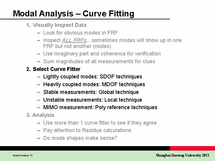
Modal Analysis – Curve Fitting 1. Visually Inspect Data – Look for obvious modes in FRF – Inspect ALL FRFs…sometimes modes will show up in one FRF but not another (nodes) – Use Imaginary part and coherence for verification – Sum magnitudes of all measurements for clues 2. Select Curve Fitter – Lightly coupled modes: SDOF techniques – Heavily coupled modes: MDOF techniques – Stable measurements: Global technique – Unstable measurements: Local technique – MIMO measurement: Poly reference techniques 3. Analysis – Use more than 1 curve fitter to see if they agree – Pay attention to Residue calculations – Do mode shapes make sense? Modal Analysis 74 Shanghai Jiaotong University 2011

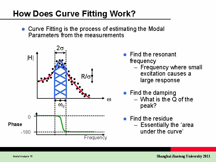
How Does Curve Fitting Work? l Curve Fitting is the process of estimating the Modal Parameters from the measurements 2 s H l Find the resonant frequency – Frequency where small excitation causes a large response l Find the damping – What is the Q of the peak? l Find the residue – Essentially the ‘area under the curve’ R/s d 0 Phase -180 Frequency Modal Analysis 75 Shanghai Jiaotong University 2011

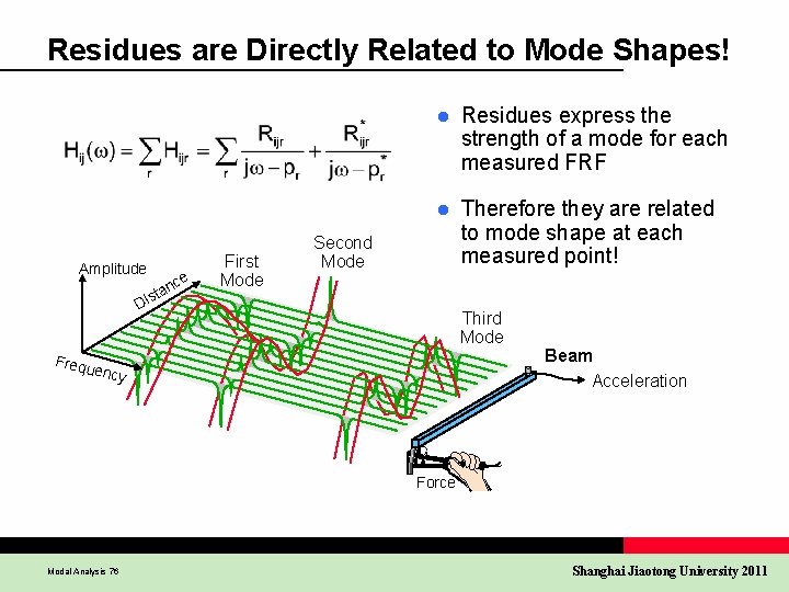
Residues are Directly Related to Mode Shapes! Amplitude Dis ce n a t Frequ e ncy First Mode Second Mode l Residues express the strength of a mode for each measured FRF l Therefore they are related to mode shape at each measured point! Third Mode Beam Acceleration Force Force Force Modal Analysis 76 Shanghai Jiaotong University 2011

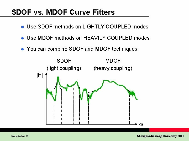
SDOF vs. MDOF Curve Fitters l Use SDOF methods on LIGHTLY COUPLED modes l Use MDOF methods on HEAVILY COUPLED modes l You can combine SDOF and MDOF techniques! SDOF (light coupling) MDOF (heavy coupling) H Modal Analysis 77 Shanghai Jiaotong University 2011

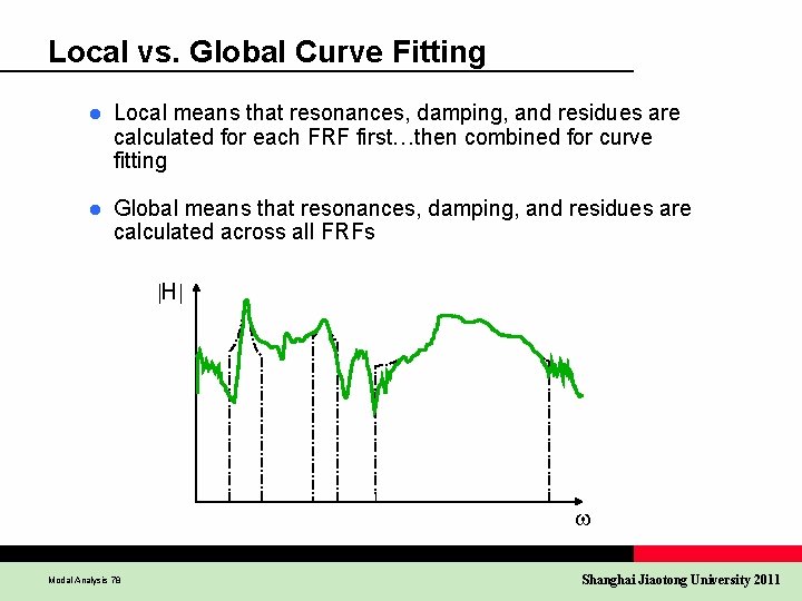
Local vs. Global Curve Fitting l Local means that resonances, damping, and residues are calculated for each FRF first…then combined for curve fitting l Global means that resonances, damping, and residues are calculated across all FRFs H Modal Analysis 78 Shanghai Jiaotong University 2011

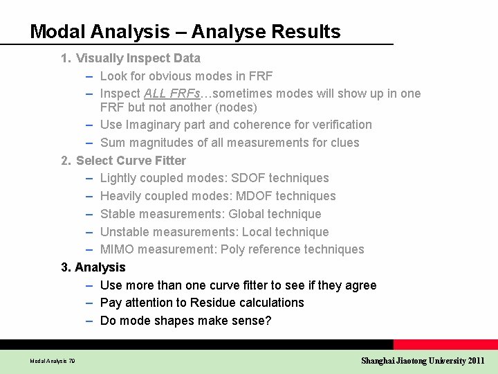
Modal Analysis – Analyse Results 1. Visually Inspect Data – Look for obvious modes in FRF – Inspect ALL FRFs…sometimes modes will show up in one FRF but not another (nodes) – Use Imaginary part and coherence for verification – Sum magnitudes of all measurements for clues 2. Select Curve Fitter – Lightly coupled modes: SDOF techniques – Heavily coupled modes: MDOF techniques – Stable measurements: Global technique – Unstable measurements: Local technique – MIMO measurement: Poly reference techniques 3. Analysis – Use more than one curve fitter to see if they agree – Pay attention to Residue calculations – Do mode shapes make sense? Modal Analysis 79 Shanghai Jiaotong University 2011

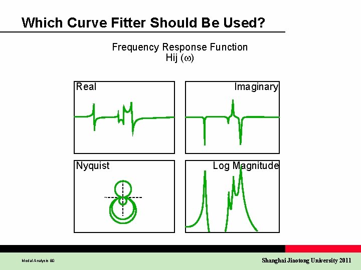
Which Curve Fitter Should Be Used? Frequency Response Function Hij ( ) Real Nyquist Modal Analysis 80 Imaginary Log Magnitude Shanghai Jiaotong University 2011

Which Curve Fitter Should Be Used? Frequency Response Function Hij ( ) Real Nyquist Modal Analysis 81 Imaginary Log Magnitude Shanghai Jiaotong University 2011

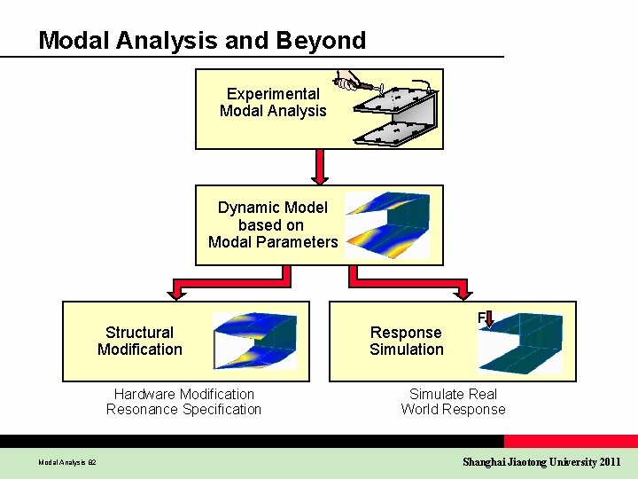
Modal Analysis and Beyond Experimental Modal Analysis Dynamic Model based on Modal Parameters Structural Modification Hardware Modification Resonance Specification Modal Analysis 82 Response Simulation F Simulate Real World Response Shanghai Jiaotong University 2011

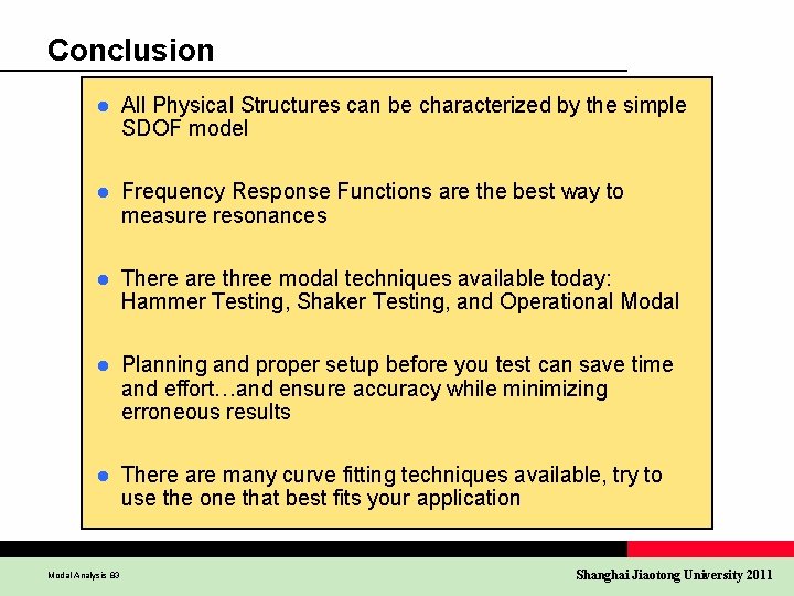
Conclusion l All Physical Structures can be characterized by the simple SDOF model l Frequency Response Functions are the best way to measure resonances l There are three modal techniques available today: Hammer Testing, Shaker Testing, and Operational Modal l Planning and proper setup before you test can save time and effort…and ensure accuracy while minimizing erroneous results l There are many curve fitting techniques available, try to use the one that best fits your application Modal Analysis 83 Shanghai Jiaotong University 2011

Literature for Further Reading l Structural Testing Part 1: Mechanical Mobility Measurements Brüel & Kjær Primer l Structural Testing Part 2: Modal Analysis and Simulation Brüel & Kjær Primer l Modal Testing: Theory, Practice, and Application, 2 nd Edition by D. J. Ewin Research Studies Press Ltd. l Dual Channel FFT Analysis (Part 1) Brüel & Kjær Technical Review # 1 – 1984 l Dual Channel FFT Analysis (Part 1) Brüel & Kjær Technical Review # 2 – 1984 Modal Analysis 84 Shanghai Jiaotong University 2011

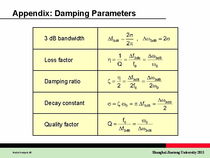
Appendix: Damping Parameters 3 d. B bandwidth , Loss factor Damping ratio Decay constant Quality factor Modal Analysis 85 Shanghai Jiaotong University 2011

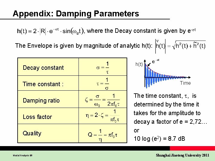
Appendix: Damping Parameters , where the Decay constant is given by e-st The Envelope is given by magnitude of analytic h(t): Decay constant Time constant : Damping ratio Loss factor Quality Modal Analysis 86 h(t) Time The time constant, t, is determined by the time it takes for the amplitude to decay a factor of e = 2, 72… or 10 log (e 2) = 8. 7 d. B Shanghai Jiaotong University 2011