Experimental Design The sampling plan or experimental design

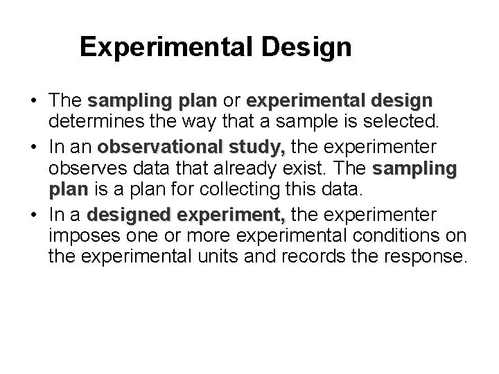
Experimental Design • The sampling plan or experimental design determines the way that a sample is selected. • In an observational study, the experimenter observes data that already exist. The sampling plan is a plan for collecting this data. • In a designed experiment, the experimenter imposes one or more experimental conditions on the experimental units and records the response.

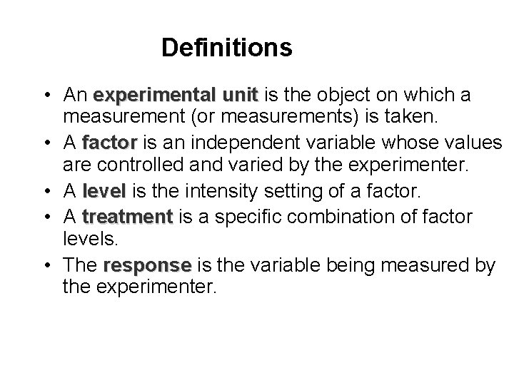
Definitions • An experimental unit is the object on which a measurement (or measurements) is taken. • A factor is an independent variable whose values are controlled and varied by the experimenter. • A level is the intensity setting of a factor. • A treatment is a specific combination of factor levels. • The response is the variable being measured by the experimenter.

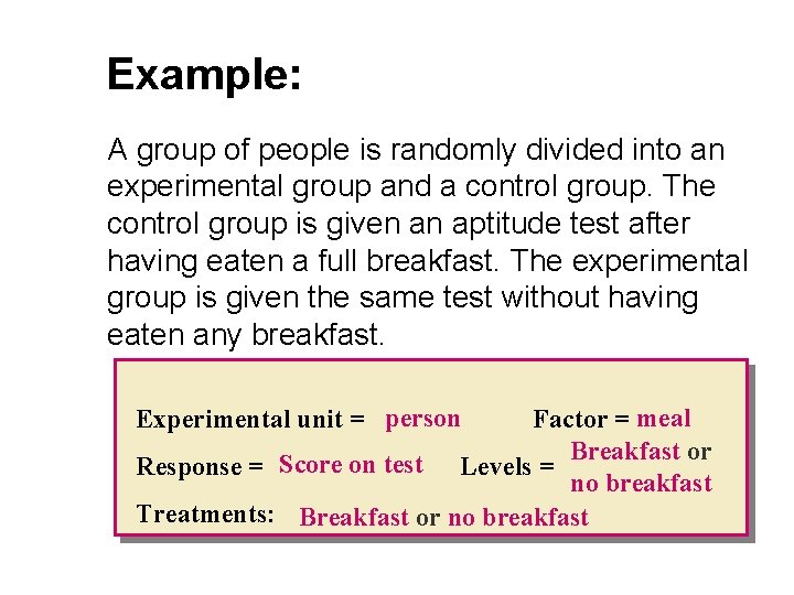
Example: A group of people is randomly divided into an experimental group and a control group. The control group is given an aptitude test after having eaten a full breakfast. The experimental group is given the same test without having eaten any breakfast. Experimental unit = person Factor = meal Breakfast or Response = Score on test Levels = no breakfast Treatments: Breakfast or no breakfast

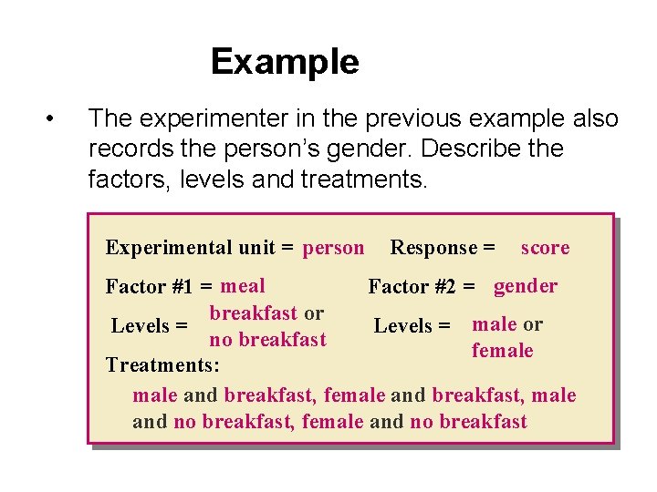
Example • The experimenter in the previous example also records the person’s gender. Describe the factors, levels and treatments. Experimental unit = person Response = score Factor #1 = meal Factor #2 = gender breakfast or Levels = male or no breakfast female Treatments: male and breakfast, female and breakfast, male and no breakfast, female and no breakfast

The Analysis of Variance (ANOVA) • All measurements exhibit variability. • The total variation in the response measurements is broken into portions that can be attributed to various factors • These portions are used to judge the effect of the various factors on the experimental response.

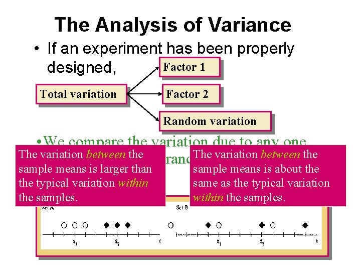
The Analysis of Variance • If an experiment has been properly Factor 1 designed, Total variation Factor 2 Random variation • We compare the variation due to any one Thefactor variationtobetween the The variation between the typical random variation in the sample means is larger than sample means is about the experiment. the typical variation within same as the typical variation the samples. within the samples.

Assumptions 1. The observations within each population are normally distributed with a common variance s 2. 2. Assumptions regarding the sampling procedures are specified for each design. • Analysis of variance procedures are fairly robust when sample sizes are equal and when the data are fairly mound-shaped.

Three Designs • • • Completely randomized design: an extension of the two independent sample t-test. Randomized block design: an extension of the paired difference test. a × b Factorial experiment: we study two experimental factors and their effect on the response.

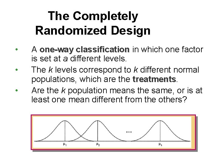
The Completely Randomized Design • • • A one-way classification in which one factor is set at a different levels. The k levels correspond to k different normal populations, which are the treatments Are the k population means the same, or is at least one mean different from the others?

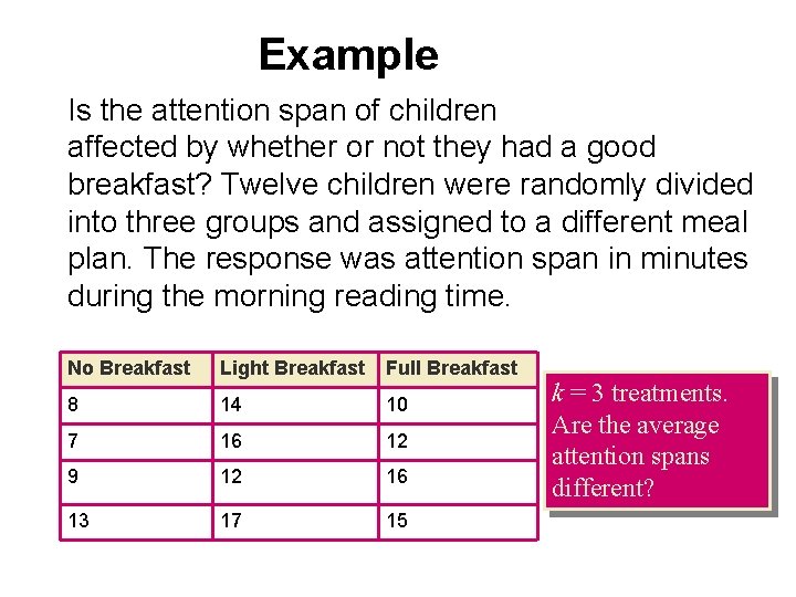
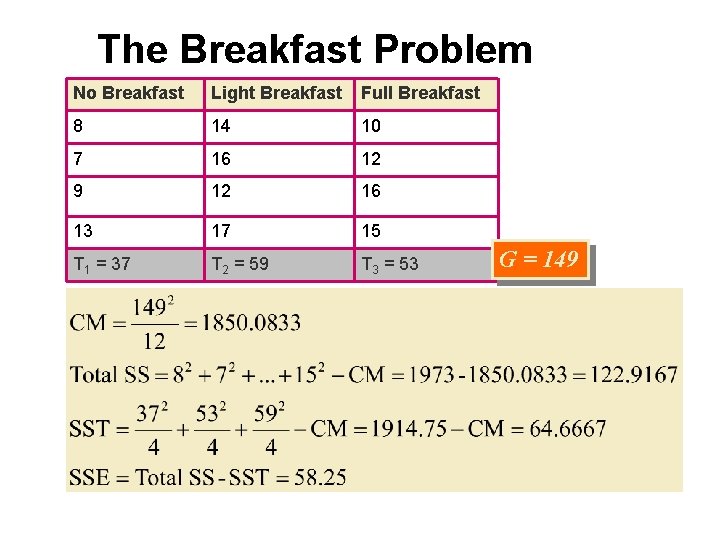
Example Is the attention span of children affected by whether or not they had a good breakfast? Twelve children were randomly divided into three groups and assigned to a different meal plan. The response was attention span in minutes during the morning reading time. No Breakfast Light Breakfast Full Breakfast 8 14 10 7 16 12 9 12 16 13 17 15 k = 3 treatments. Are the average attention spans different?

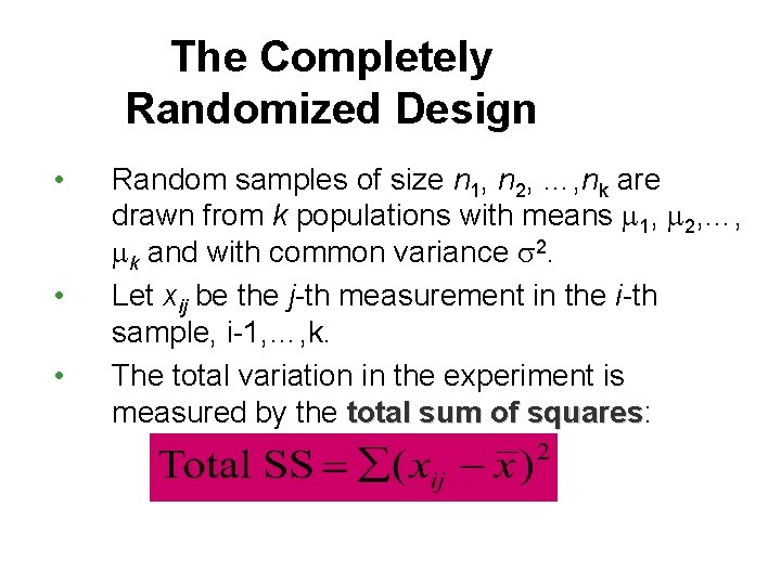
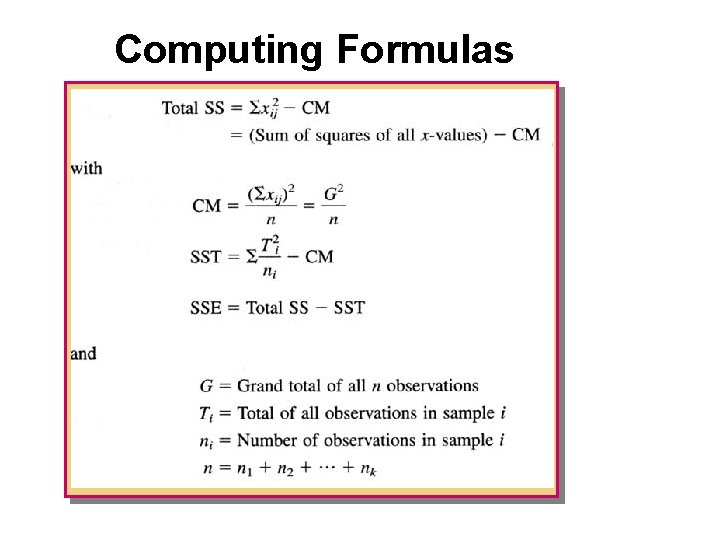
The Completely Randomized Design • • • Random samples of size n 1, n 2, …, nk are drawn from k populations with means m 1, m 2, …, mk and with common variance s 2. Let xij be the j-th measurement in the i-th sample, i-1, …, k. The total variation in the experiment is measured by the total sum of squares: squares

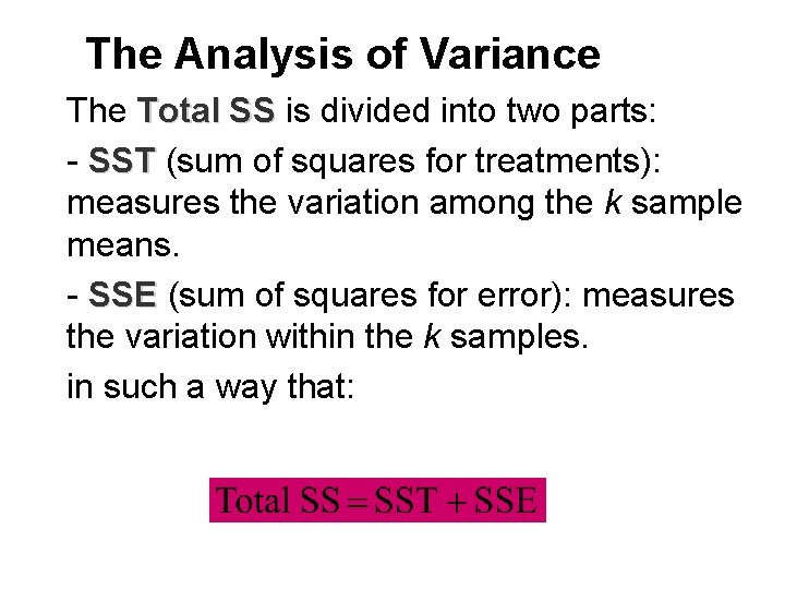
The Analysis of Variance The Total SS is divided into two parts: - SST (sum of squares for treatments): measures the variation among the k sample means. - SSE (sum of squares for error): measures the variation within the k samples. in such a way that:

Computing Formulas

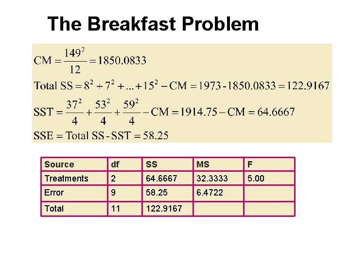
The Breakfast Problem No Breakfast Light Breakfast Full Breakfast 8 14 10 7 16 12 9 12 16 13 17 15 T 1 = 37 T 2 = 59 T 3 = 53 G = 149

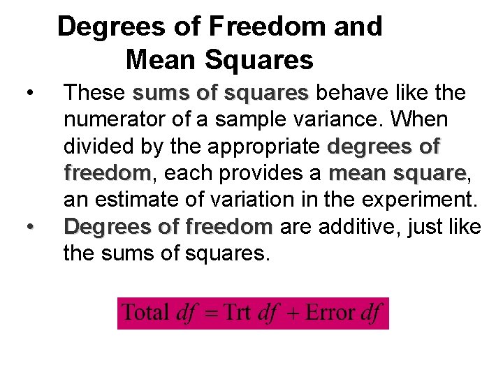
Degrees of Freedom and Mean Squares • • These sums of squares behave like the numerator of a sample variance. When divided by the appropriate degrees of freedom, freedom each provides a mean square, square an estimate of variation in the experiment. Degrees of freedom are additive, just like the sums of squares.

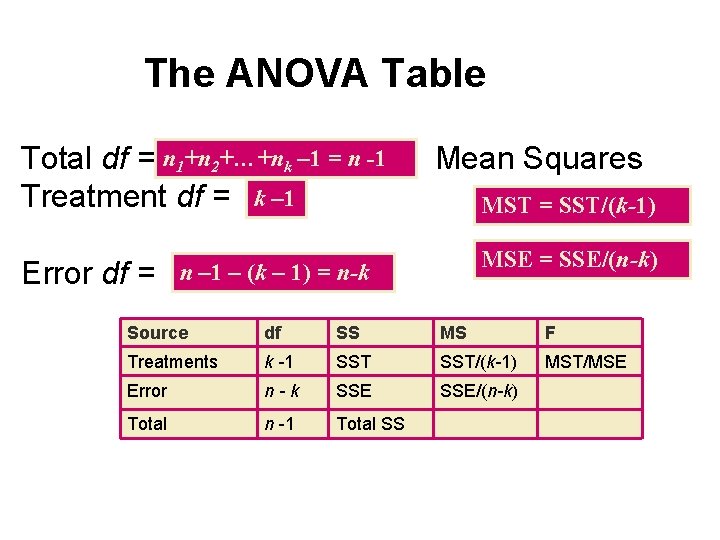
The ANOVA Table Total df = n 1+n 2+…+nk – 1 = n -1 Treatment df = k – 1 Error df = Mean Squares MST = SST/(k-1) MSE = SSE/(n-k) n – 1 – (k – 1) = n-k Source df SS MS F Treatments k -1 SST/(k-1) MST/MSE Error n-k SSE/(n-k) Total n -1 Total SS

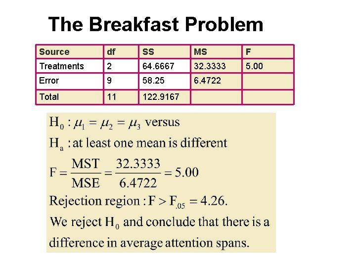
The Breakfast Problem Source df SS MS F Treatments 2 64. 6667 32. 3333 5. 00 Error 9 58. 25 6. 4722 Total 11 122. 9167

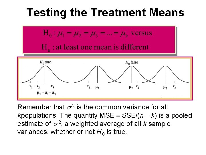
Testing the Treatment Means Remember that s 2 is the common variance for all kpopulations. The quantity MSE = SSE/(n - k) is a pooled estimate of s 2, a weighted average of all k sample variances, whether or not H 0 is true.

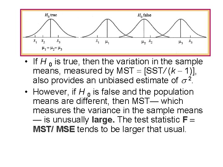
• If H 0 is true, then the variation in the sample means, measured by MST = [SST/ (k - 1)], also provides an unbiased estimate of s 2. • However, if H 0 is false and the population means are different, then MST— which measures the variance in the sample means — is unusually large. The test statistic F = MST/ MSE tends to be larger that usual.

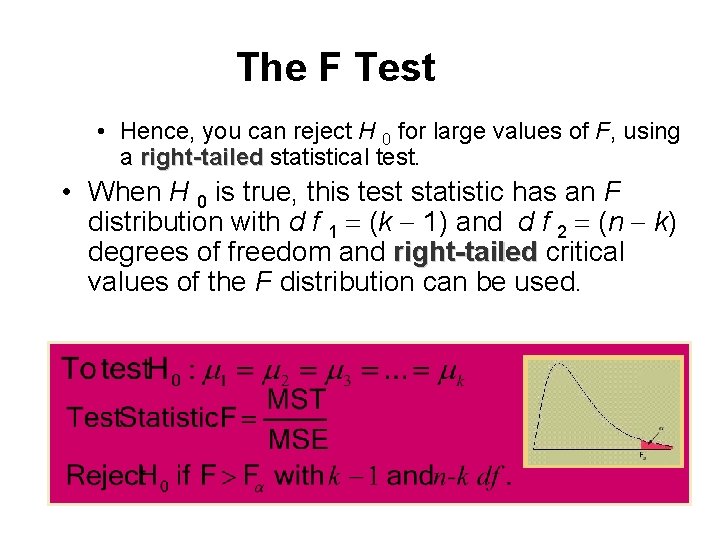
The F Test • Hence, you can reject H 0 for large values of F, using a right-tailed statistical test. • When H 0 is true, this test statistic has an F distribution with d f 1 = (k - 1) and d f 2 = (n - k) degrees of freedom and right-tailed critical values of the F distribution can be used.

The Breakfast Problem Source df SS MS F Treatments 2 64. 6667 32. 3333 5. 00 Error 9 58. 25 6. 4722 Total 11 122. 9167

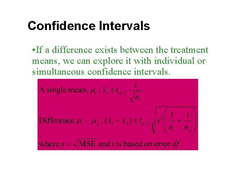
Confidence Intervals • If a difference exists between the treatment means, we can explore it with individual or simultaneous confidence intervals.

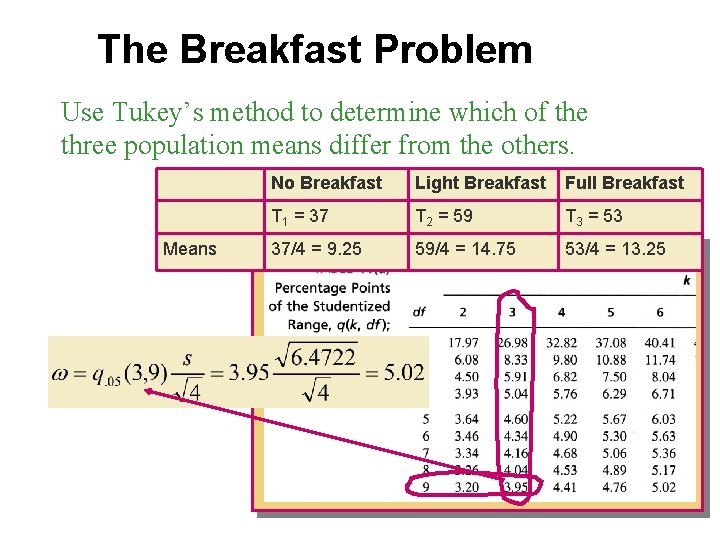
Tukey’s Method for Paired Comparisons • Designed to test all pairs of population means simultaneously, with an overall error rate of a. • Based on the studentized range, range the difference between the largest and smallest of the k sample means. • Assume that the sample sizes are equal and calculate a “ruler” that measures the distance required between any pair of means to declare a significant difference.

Tukey’s Method

The Breakfast Problem Use Tukey’s method to determine which of the three population means differ from the others. Means No Breakfast Light Breakfast Full Breakfast T 1 = 37 T 2 = 59 T 3 = 53 37/4 = 9. 25 59/4 = 14. 75 53/4 = 13. 25

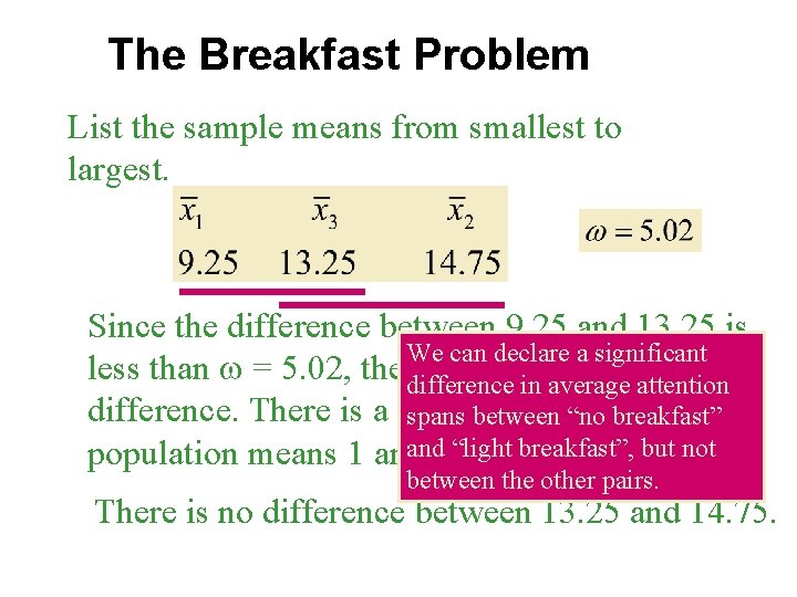
The Breakfast Problem List the sample means from smallest to largest. Since the difference between 9. 25 and 13. 25 is We can declare a significant less than w = 5. 02, there is no significant difference in average attention difference. There is a difference spans between “no breakfast” and 2“light breakfast”, but not population means 1 and however. between the other pairs. There is no difference between 13. 25 and 14. 75.

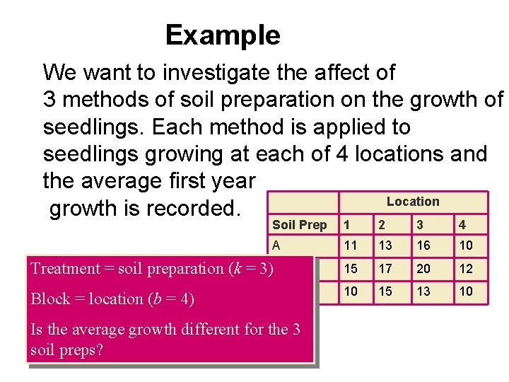
The Randomized Block Design • • • A direct extension of the paired difference or matched pairs design. A two-way classification in which k treatment means are compared. The design uses blocks of k experimental units that are relatively similar or homogeneous, with one unit within each block randomly assigned to each treatment.

The Randomized Block Design • • • If the design involves k treatments within each of b blocks, blocks then the total number of observations is n = bk. bk The purpose of blocking is to remove or isolate the block-to-block variability that might hide the effect of the treatments. There are two factors—treatments and blocks, blocks only one of which is of interest to the expeirmenter.

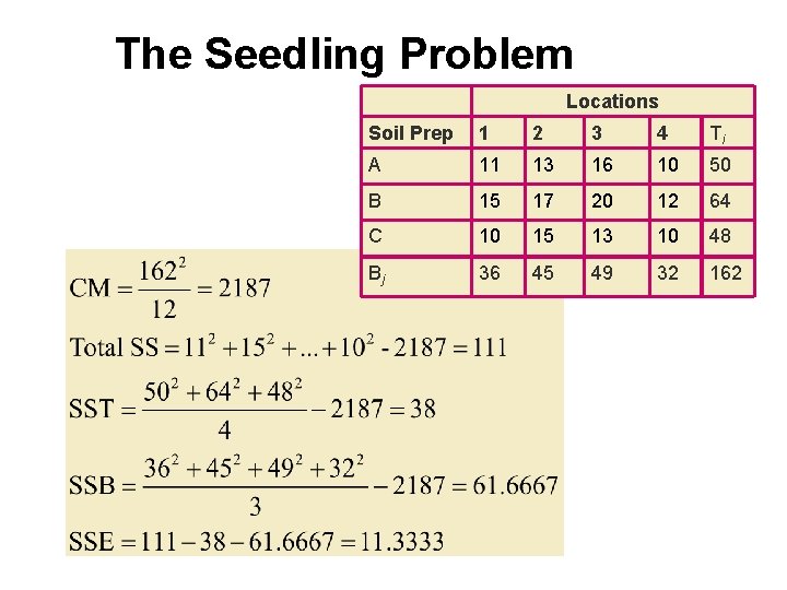
Example We want to investigate the affect of 3 methods of soil preparation on the growth of seedlings. Each method is applied to seedlings growing at each of 4 locations and the average first year Location growth is recorded. Soil Prep 1 2 3 4 A 11 13 16 10 Treatment = soil preparation (k = 3)B 15 17 20 12 C 10 15 13 10 Block = location (b = 4) Is the average growth different for the 3 soil preps?

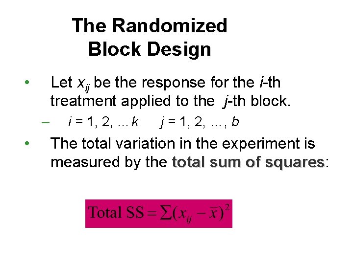
The Randomized Block Design • Let xij be the response for the i-th treatment applied to the j-th block. – • i = 1, 2, …k j = 1, 2, …, b The total variation in the experiment is measured by the total sum of squares: squares

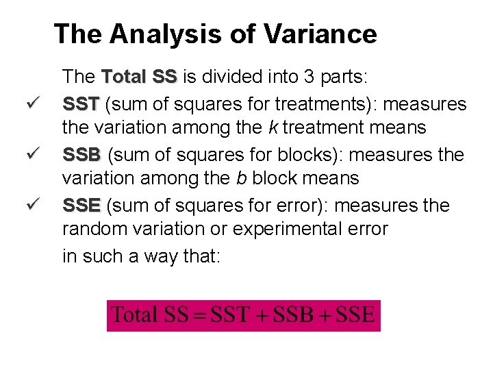
The Analysis of Variance ü ü ü The Total SS is divided into 3 parts: SST (sum of squares for treatments): measures the variation among the k treatment means SSB (sum of squares for blocks): measures the variation among the b block means SSE (sum of squares for error): measures the random variation or experimental error in such a way that:

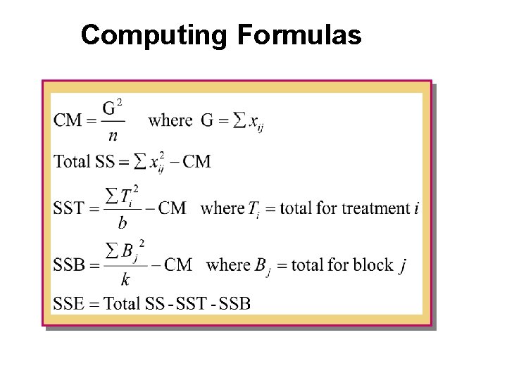
Computing Formulas

The Seedling Problem Locations Soil Prep 1 2 3 4 Ti A 11 13 16 10 50 B 15 17 20 12 64 C 10 15 13 10 48 Bj 36 45 49 32 162

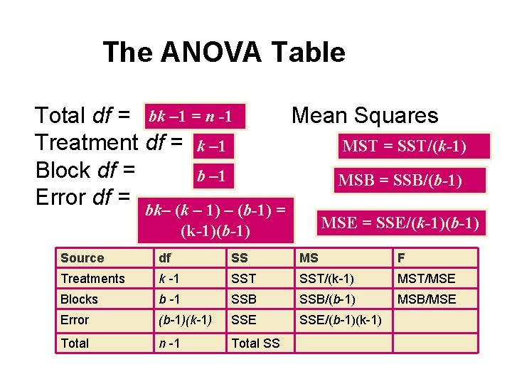
The ANOVA Table Total df = bk – 1 = n -1 Mean Squares Treatment df = k – 1 MST = SST/(k-1) Block df = b – 1 MSB = SSB/(b-1) Error df = bk– (k – 1) – (b-1) = MSE = SSE/(k-1)(b-1) Source df SS MS F Treatments k -1 SST/(k-1) MST/MSE Blocks b -1 SSB/(b-1) MSB/MSE Error (b-1)(k-1) SSE/(b-1)(k-1) Total n -1 Total SS

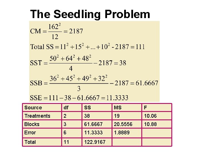
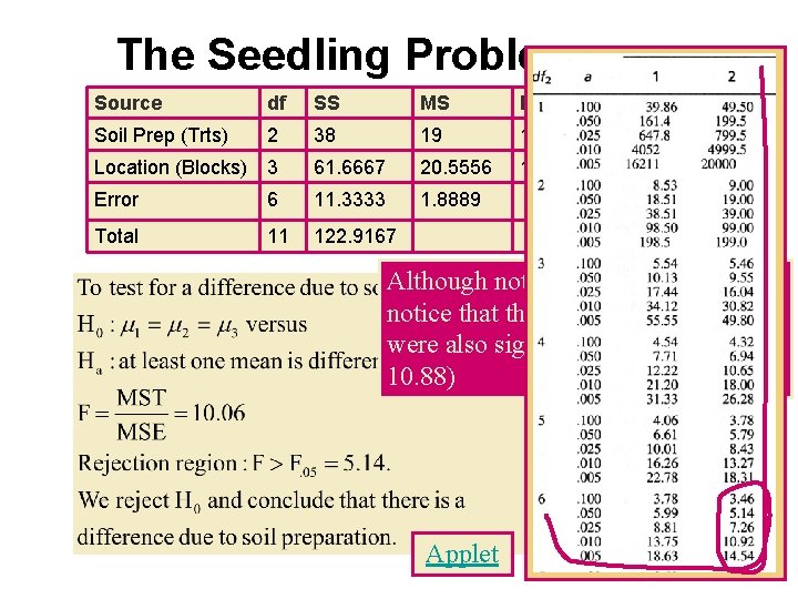
The Seedling Problem Source df SS MS F Treatments 2 38 19 10. 06 Blocks 3 61. 6667 20. 5556 10. 88 Error 6 11. 3333 1. 8889 Total 11 122. 9167

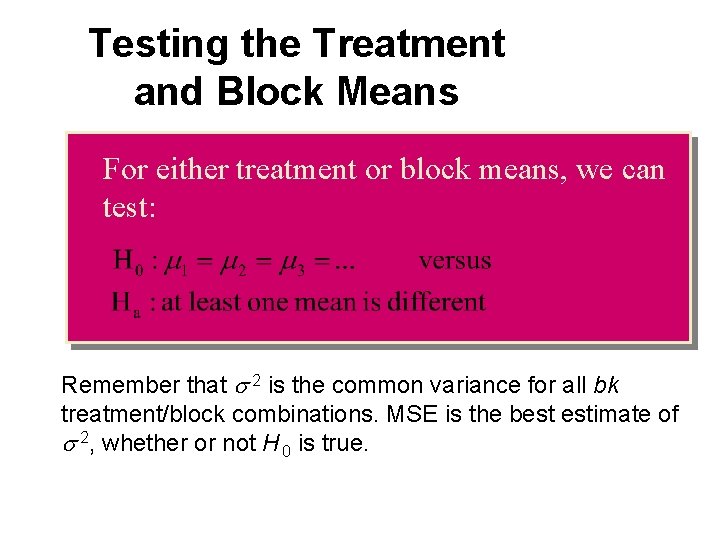
Testing the Treatment and Block Means For either treatment or block means, we can test: Remember that s 2 is the common variance for all bk treatment/block combinations. MSE is the best estimate of s 2, whether or not H 0 is true.

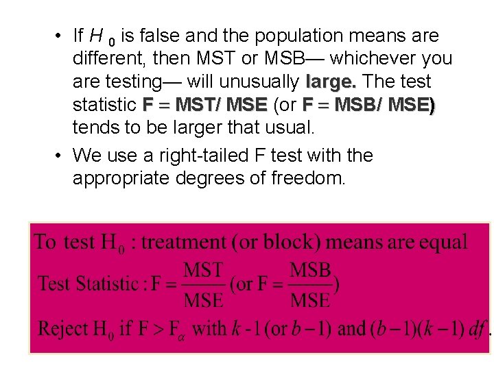
• If H 0 is false and the population means are different, then MST or MSB— whichever you are testing— will unusually large. The test statistic F = MST/ MSE (or F = MSB/ MSE) tends to be larger that usual. • We use a right-tailed F test with the appropriate degrees of freedom.

The Seedling Problem Source df SS MS F Soil Prep (Trts) 2 38 19 10. 06 Location (Blocks) 3 61. 6667 20. 5556 10. 88 Error 6 11. 3333 1. 8889 Total 11 122. 9167 Although not of primary importance, notice that the blocks (locations) were also significantly different (F = 10. 88) Applet

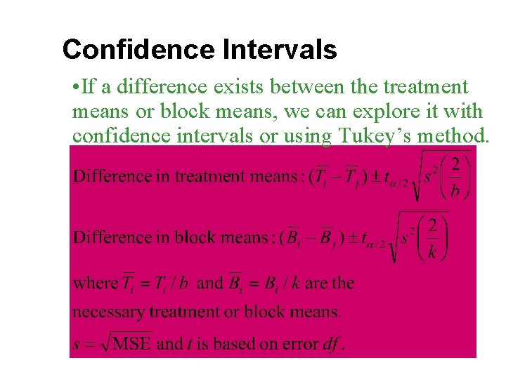
Confidence Intervals • If a difference exists between the treatment means or block means, we can explore it with confidence intervals or using Tukey’s method.

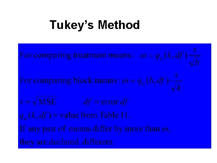
Tukey’s Method

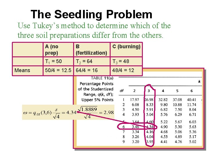
The Seedling Problem Use Tukey’s method to determine which of the three soil preparations differ from the others. Means A (no prep) B C (burning) (fertilization) T 1 = 50 T 2 = 64 50/4 = 12. 5 64/4 = 16 T 3 = 48 48/4 = 12

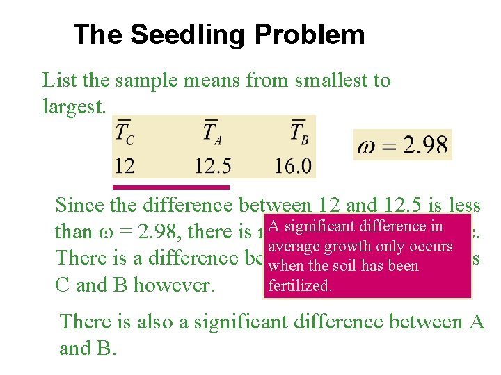
The Seedling Problem List the sample means from smallest to largest. Since the difference between 12 and 12. 5 is less A significant difference in than w = 2. 98, there is no significant difference. average growth only occurs There is a difference between when thepopulation soil has been means fertilized. C and B however. There is also a significant difference between A and B.

Cautions about Blocking üA randomized block design should not be used when treatments and blocks both correspond to experimental factors of interest to the researcher üRemember that blocking may not always be beneficial. üRemember that you cannot construct confidence intervals for individual treatment means unless it is reasonable to assume that the b blocks have been randomly selected from a population of blocks.

An a x b Factorial Experiment • • • A two-way classification in which involves two factors, both of which are of interest to the experimenter. There a levels of factor A and b levels of factor B—the experiment is replicated r times at each factor-level combination. The replications allow the experimenter to investigate the interaction between factors A and B.

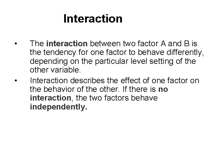
Interaction • • The interaction between two factor A and B is the tendency for one factor to behave differently, depending on the particular level setting of the other variable. Interaction describes the effect of one factor on the behavior of the other. If there is no interaction, the two factors behave independently.

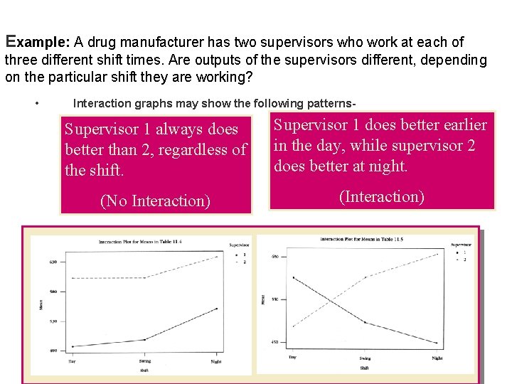
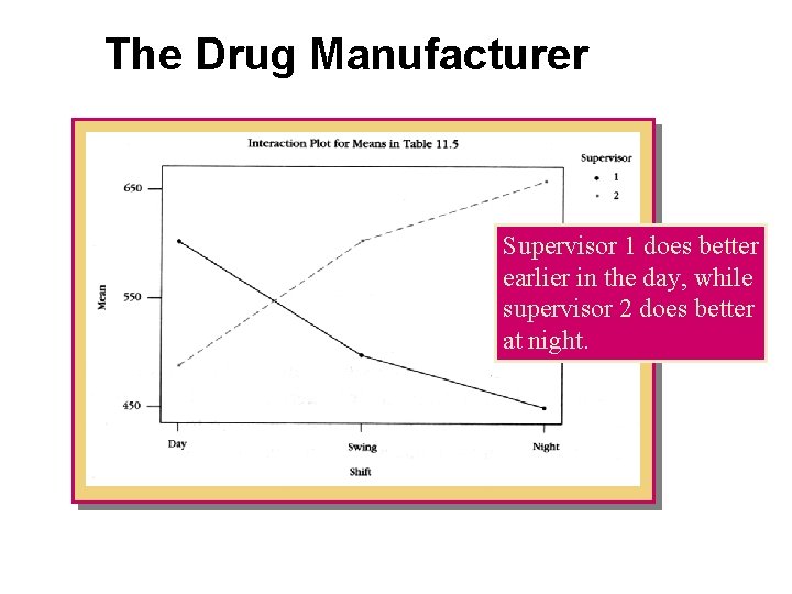
Example: A drug manufacturer has two supervisors who work at each of three different shift times. Are outputs of the supervisors different, depending on the particular shift they are working? • Interaction graphs may show the following patterns- Supervisor 1 always does better than 2, regardless of the shift. Supervisor 1 does better earlier in the day, while supervisor 2 does better at night. (No Interaction) (Interaction)

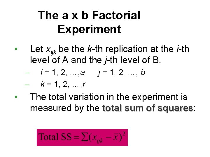
The a x b Factorial Experiment • Let xijk be the k-th replication at the i-th level of A and the j-th level of B. – – • i = 1, 2, …, a k = 1, 2, …, r j = 1, 2, …, b The total variation in the experiment is measured by the total sum of squares: squares

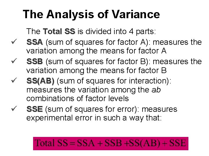
The Analysis of Variance ü ü The Total SS is divided into 4 parts: SSA (sum of squares for factor A): measures the variation among the means for factor A SSB (sum of squares for factor B): measures the variation among the means for factor B SS(AB) (sum of squares for interaction): measures the variation among the ab combinations of factor levels SSE (sum of squares for error): measures experimental error in such a way that:

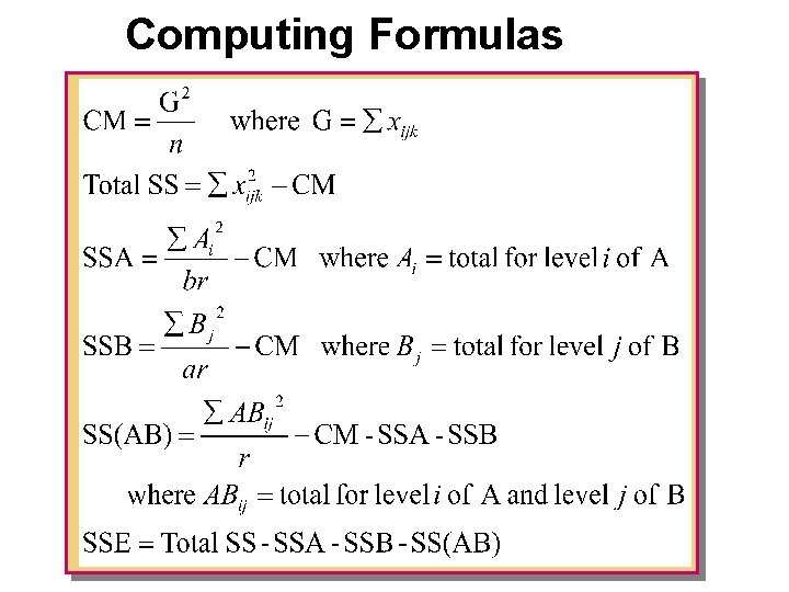
Computing Formulas

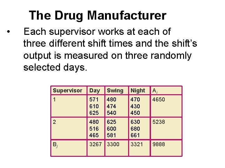
The Drug Manufacturer • Each supervisor works at each of three different shift times and the shift’s output is measured on three randomly selected days. Supervisor Day Swing Night Ai 1 571 610 625 480 474 540 470 430 450 4650 2 480 516 465 625 600 581 630 680 661 5238 Bj 3267 3300 3321 9888

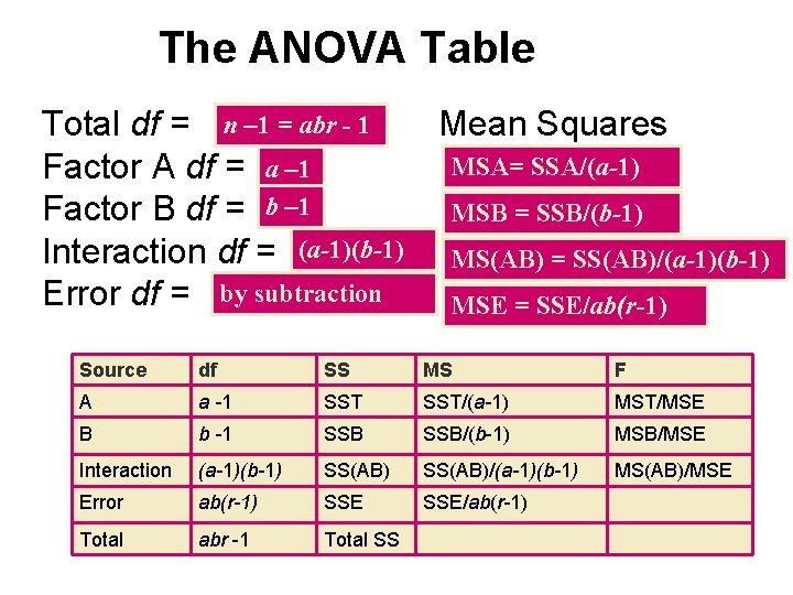
The ANOVA Table Total df = n – 1 = abr - 1 Mean Squares MSA= SSA/(a-1) Factor A df = a – 1 Factor B df = b – 1 MSB = SSB/(b-1) Interaction df = (a-1)(b-1) MS(AB) = SS(AB)/(a-1)(b-1) Error df = by subtraction MSE = SSE/ab(r-1) Source df SS MS F A a -1 SST/(a-1) MST/MSE B b -1 SSB/(b-1) MSB/MSE Interaction (a-1)(b-1) SS(AB)/(a-1)(b-1) MS(AB)/MSE Error ab(r-1) SSE/ab(r-1) Total abr -1 Total SS

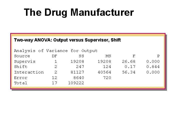
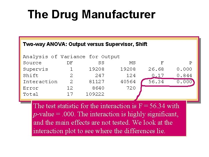
The Drug Manufacturer Two-way ANOVA: Output versus Supervisor, Shift Analysis of Variance for Output Source DF SS MS Supervis 1 19208 Shift 2 247 124 Interaction 2 81127 40564 Error 12 8640 720 Total 17 109222 F 26. 68 0. 17 56. 34 P 0. 000 0. 844 0. 000

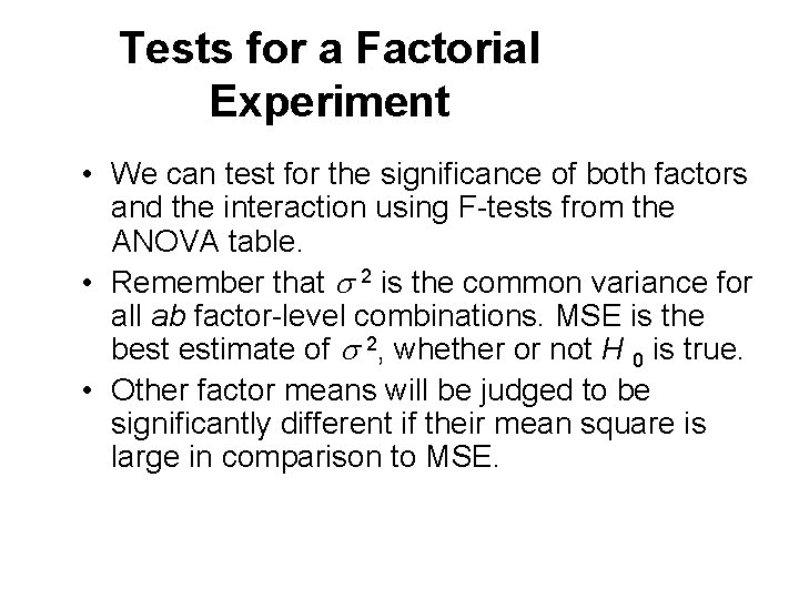
Tests for a Factorial Experiment • We can test for the significance of both factors and the interaction using F-tests from the ANOVA table. • Remember that s 2 is the common variance for all ab factor-level combinations. MSE is the best estimate of s 2, whether or not H 0 is true. • Other factor means will be judged to be significantly different if their mean square is large in comparison to MSE.

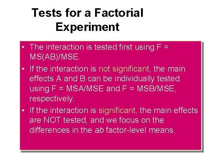
Tests for a Factorial Experiment • The interaction is tested first using F = MS(AB)/MSE. • If the interaction is not significant, the main effects A and B can be individually tested using F = MSA/MSE and F = MSB/MSE, respectively. • If the interaction is significant, the main effects are NOT tested, and we focus on the differences in the ab factor-level means.

The Drug Manufacturer Two-way ANOVA: Output versus Supervisor, Shift Analysis of Variance for Output Source DF SS MS Supervis 1 19208 Shift 2 247 124 Interaction 2 81127 40564 Error 12 8640 720 Total 17 109222 F 26. 68 0. 17 56. 34 P 0. 000 0. 844 0. 000 The test statistic for the interaction is F = 56. 34 with p-value =. 000. The interaction is highly significant, and the main effects are not tested. We look at the interaction plot to see where the differences lie.

The Drug Manufacturer Supervisor 1 does better earlier in the day, while supervisor 2 does better at night.

Revisiting the ANOVA Assumptions 1. The observations within each population are normally distributed with a common variance s 2. 2. Assumptions regarding the sampling procedures are specified for each design. • Remember that ANOVA procedures are fairly robust when sample sizes are equal and when the data are fairly mound-shaped.

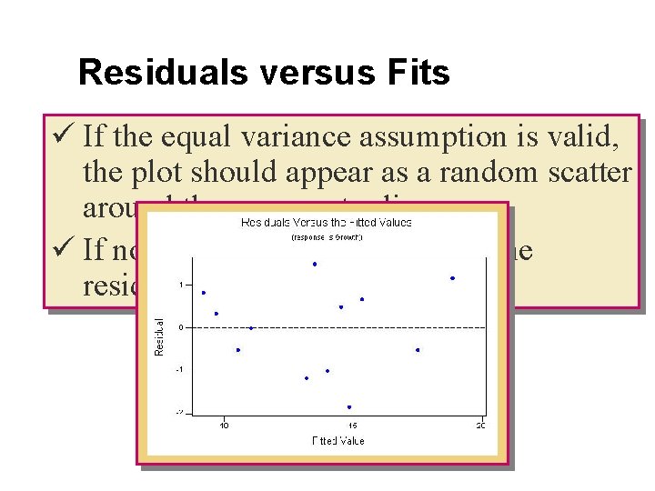
Diagnostic Tools • Many computer programs have graphics options that allow you to check the normality assumption and the assumption of equal variances. 1. Normal probability plot of residuals 2. Plot of residuals versus fit or residuals versus variables

Residuals • The analysis of variance procedure takes the total variation in the experiment and partitions out amounts for several important factors. • The “leftover” variation in each data point is called the residual or experimental error • If all assumptions have been met, these residuals should be normal, normal with mean 0 and variance s 2.

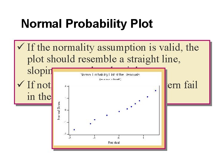
Normal Probability Plot ü If the normality assumption is valid, the plot should resemble a straight line, sloping upward to the right. ü If not, you will often see the pattern fail in the tails of the graph.

Residuals versus Fits ü If the equal variance assumption is valid, the plot should appear as a random scatter around the zero center line. ü If not, you will see a pattern in the residuals.

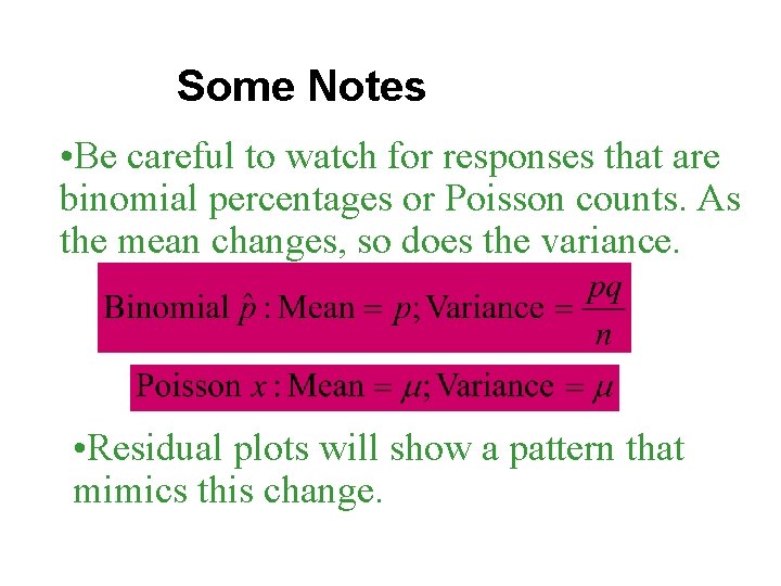
Some Notes • Be careful to watch for responses that are binomial percentages or Poisson counts. As the mean changes, so does the variance. • Residual plots will show a pattern that mimics this change.

Some Notes • Watch for missing data or a lack of randomization in the design of the experiment. • Randomized block designs with missing values and factorial experiments with unequal replications cannot be analyzed using the ANOVA formulas given in this chapter. Use multiple regression analysis instead.

Key Concepts I. Experimental Designs 1. Experimental units, factors, levels, treatments, response variables. 2. Assumptions: Observations within each treatment group must be normally distributed with a common variance s 2. 3. One-way classification—completely randomized design: Independent random samples are selected from each of k populations. 4. Two-way classification—randomized block design: k treatments are compared within b blocks. 5. Two-way classification — a ´ b factorial experiment: Two factors, A and B, are compared at several levels. Each factor– level combination is replicated r times to allow for the investigation of an interaction between the two factors.

Key Concepts II. Analysis of Variance 1. The total variation in the experiment is divided into variation (sums of squares) explained by the various experimental factors and variation due to experimental error (unexplained). 2. If there is an effect due to a particular factor, its mean square(MS = SS/df ) is usually large and F = MS(factor)/MSE is large. 3. Test statistics for the various experimental factors are based on F statistics, with appropriate degrees of freedom (d f 2 = Error degrees of freedom).

Key Concepts III. 1. 2. 3. 4. Interpreting an Analysis of Variance For the completely randomized and randomized block design, each factor is tested for significance. For the factorial experiment, first test for a significant interaction. If the interactions is significant, main effects need not be tested. The nature of the difference in the factor– level combinations should be further examined. If a significant difference in the population means is found, Tukey’s method of pairwise comparisons or a similar method can be used to further identify the nature of the difference. If you have a special interest in one population mean or the difference between two population means, you can use a confidence interval estimate. (For randomized block design, confidence intervals do not provide estimates for single population means).

Key Concepts IV. 1. 2. Checking the Analysis of Variance Assumptions To check for normality, use the normal probability plot for the residuals. The residuals should exhibit a straight-line pattern, sloping upward to the right. To check for equality of variance, use the residuals versus fit plot. The plot should exhibit a random scatter, with the same vertical spread around the horizontal “zero error line. ”