Experimental design and sample size determination Karl W

Experimental design and sample size determination Karl W Broman Department of Biostatistics Johns Hopkins University http: //www. biostat. jhsph. edu/~kbroman

Note • This is a shortened version of a lecture which is part of a webbased course on “Enhancing Humane Science/Improving Animal Research” (organized by Alan Goldberg, Johns Hopkins Center for Alternatives to Animal Testing) • Few details—mostly concepts. 2

Experimental design

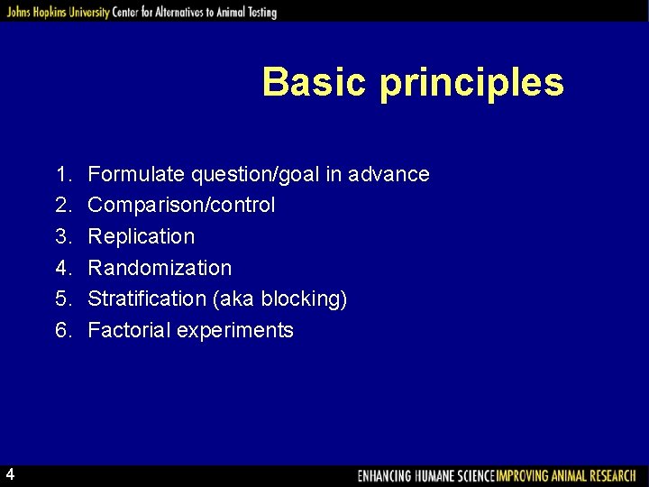
Basic principles 1. 2. 3. 4. 5. 6. 4 Formulate question/goal in advance Comparison/control Replication Randomization Stratification (aka blocking) Factorial experiments

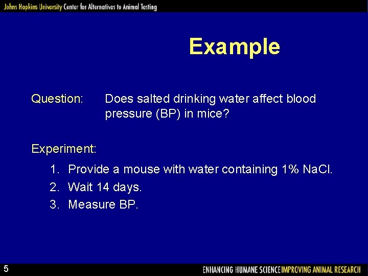
Example Question: Does salted drinking water affect blood pressure (BP) in mice? Experiment: 1. Provide a mouse with water containing 1% Na. Cl. 2. Wait 14 days. 3. Measure BP. 5

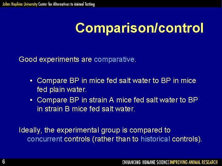
Comparison/control Good experiments are comparative. • Compare BP in mice fed salt water to BP in mice fed plain water. • Compare BP in strain A mice fed salt water to BP in strain B mice fed salt water. Ideally, the experimental group is compared to concurrent controls (rather than to historical controls). 6

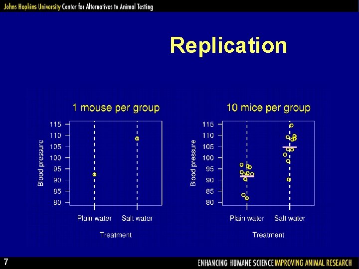
Replication 7

Why replicate? • Reduce the effect of uncontrolled variation (i. e. , increase precision). • Quantify uncertainty. A related point: An estimate is of no value without some statement of the uncertainty in the estimate. 8

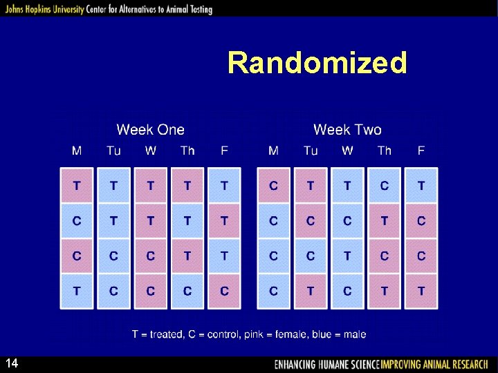
Randomization Experimental subjects (“units”) should be assigned to treatment groups at random. At random does not mean haphazardly. One needs to explicitly randomize using • A computer, or • Coins, dice or cards. 9

Why randomize? • Avoid bias. – For example: the first six mice you grab may have intrinsicly higher BP. • Control the role of chance. – Randomization allows the later use of probability theory, and so gives a solid foundation for statistical analysis. 10

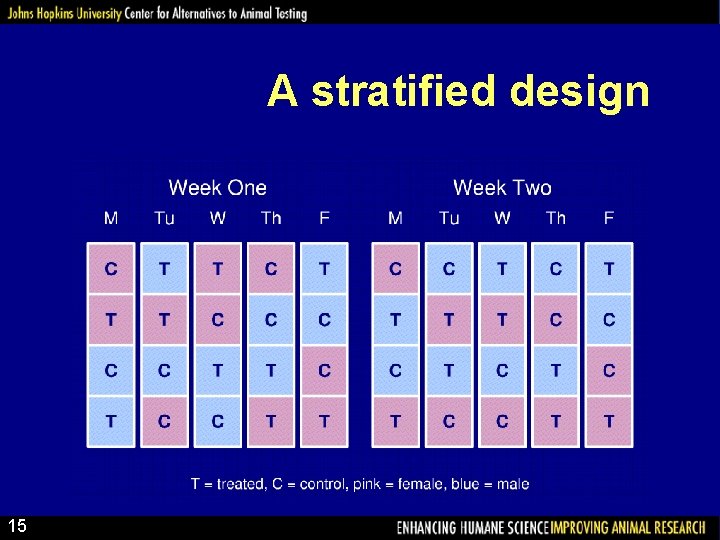
Stratification • Suppose that some BP measurements will be made in the morning and some in the afternoon. • If you anticipate a difference between morning and afternoon measurements: – Ensure that within each period, there are equal numbers of subjects in each treatment group. – Take account of the difference between periods in your analysis. • This is sometimes called “blocking”. 11

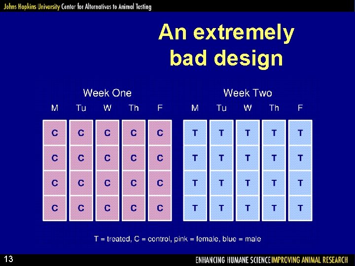
Example • 20 male mice and 20 female mice. • Half to be treated; the other half left untreated. • Can only work with 4 mice per day. Question: 12 How to assign individuals to treatment groups and to days?

An extremely bad design 13

Randomized 14

A stratified design 15

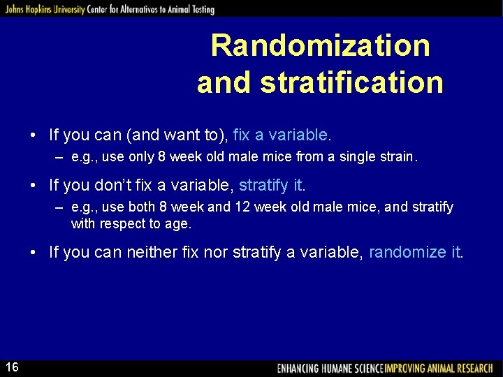
Randomization and stratification • If you can (and want to), fix a variable. – e. g. , use only 8 week old male mice from a single strain. • If you don’t fix a variable, stratify it. – e. g. , use both 8 week and 12 week old male mice, and stratify with respect to age. • If you can neither fix nor stratify a variable, randomize it. 16

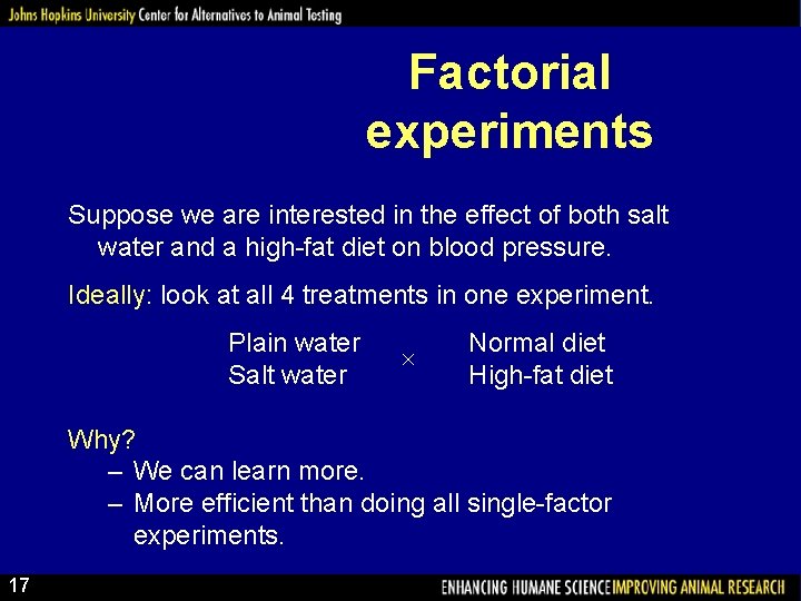
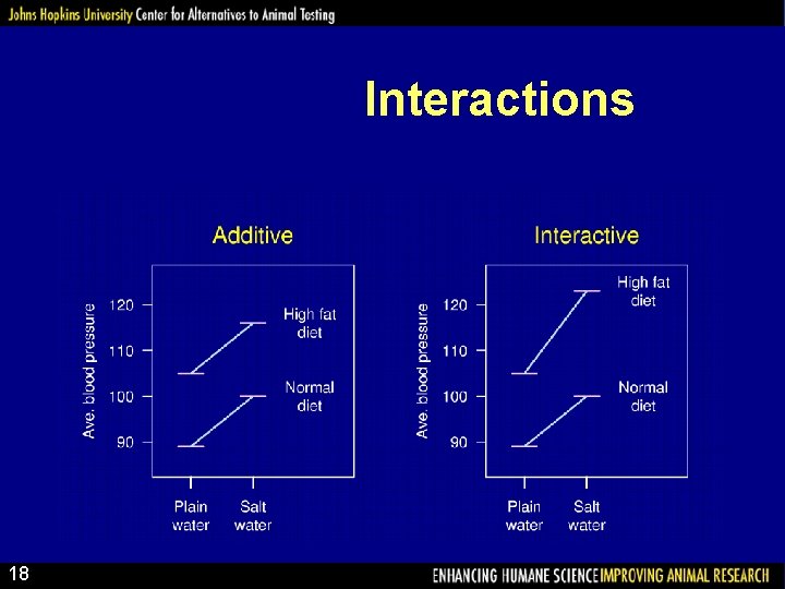
Factorial experiments Suppose we are interested in the effect of both salt water and a high-fat diet on blood pressure. Ideally: look at all 4 treatments in one experiment. Plain water Salt water Normal diet High-fat diet Why? – We can learn more. – More efficient than doing all single-factor experiments. 17

Interactions 18

Other points • Blinding – Measurements made by people can be influenced by unconscious biases. – Ideally, dissections and measurements should be made without knowledge of the treatment applied. • Internal controls – It can be useful to use the subjects themselves as their own controls (e. g. , consider the response after vs. before treatment). – Why? Increased precision. 19

Other points • Representativeness – Are the subjects/tissues you are studying really representative of the population you want to study? – Ideally, your study material is a random sample from the population of interest. 20

Summary Characteristics of good experiments: • Unbiased – Randomization – Blinding • High precision – Uniform material – Replication – Blocking • Simple – Protect against mistakes 21 • Wide range of applicability – Deliberate variation – Factorial designs • Able to estimate uncertainty – Replication – Randomization

Data presentation Good plot 22 Bad plot

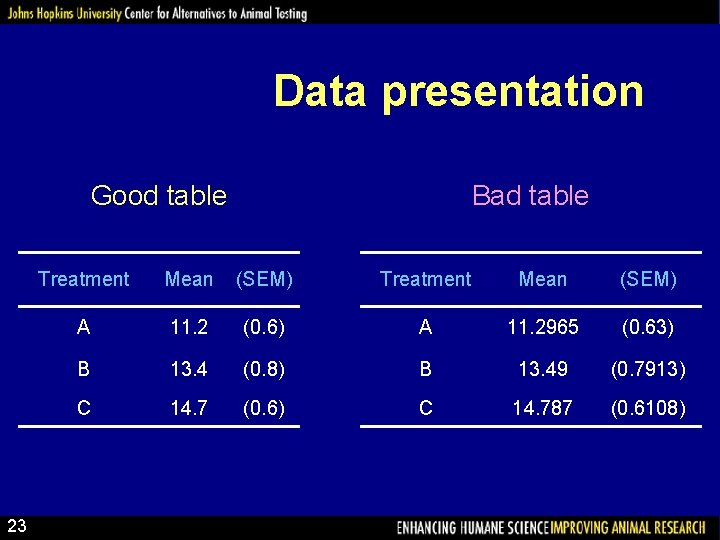
Data presentation Bad table Good table 23 Treatment Mean (SEM) A 11. 2 (0. 6) A 11. 2965 (0. 63) B 13. 4 (0. 8) B 13. 49 (0. 7913) C 14. 7 (0. 6) C 14. 787 (0. 6108)

Sample size determination

Fundamental formula 25

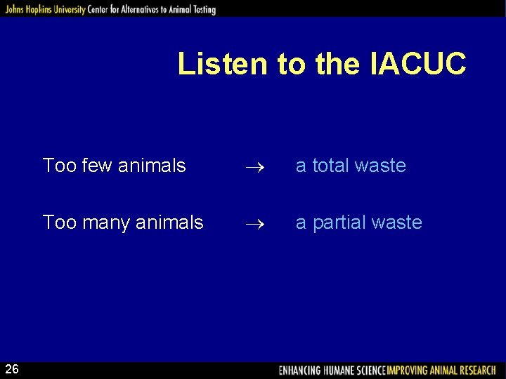
Listen to the IACUC 26 Too few animals a total waste Too many animals a partial waste

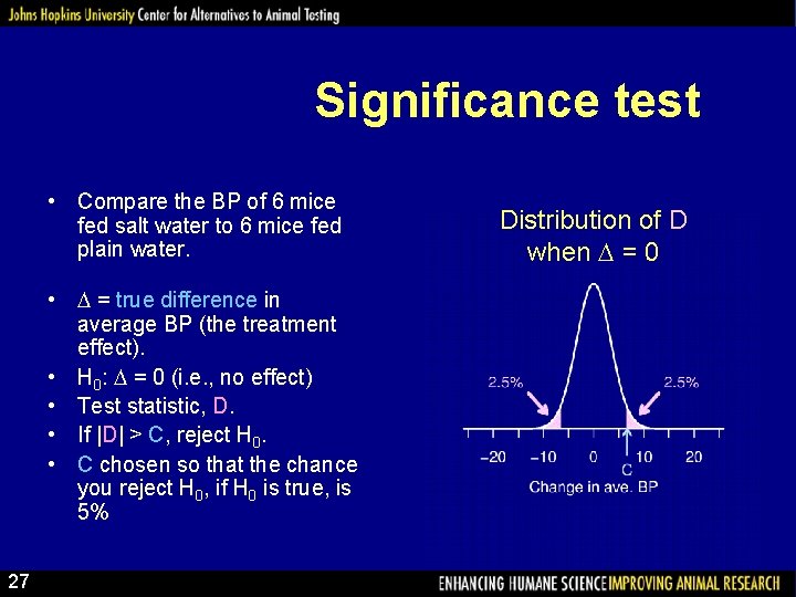
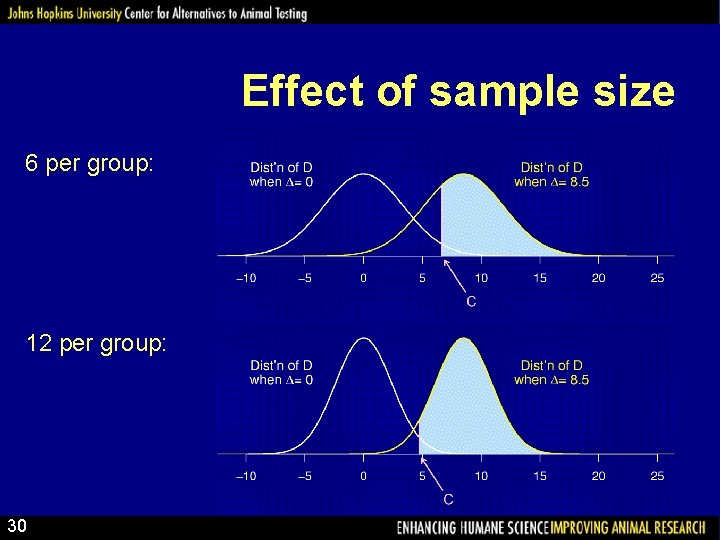
Significance test • Compare the BP of 6 mice fed salt water to 6 mice fed plain water. • = true difference in average BP (the treatment effect). • H 0: = 0 (i. e. , no effect) • Test statistic, D. • If |D| > C, reject H 0. • C chosen so that the chance you reject H 0, if H 0 is true, is 5% 27 Distribution of D when = 0

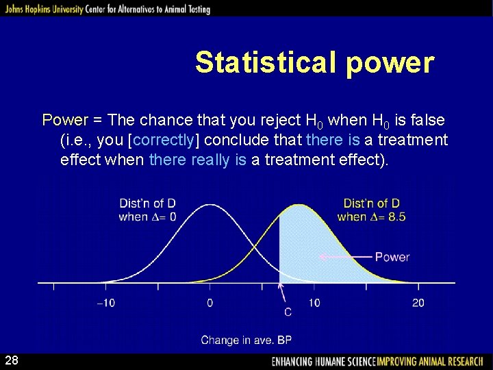
Statistical power Power = The chance that you reject H 0 when H 0 is false (i. e. , you [correctly] conclude that there is a treatment effect when there really is a treatment effect). 28

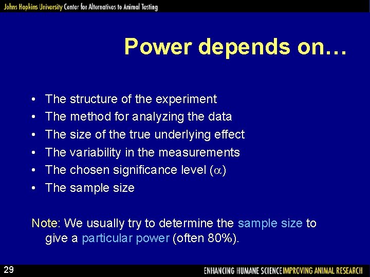
Power depends on… • • • The structure of the experiment The method for analyzing the data The size of the true underlying effect The variability in the measurements The chosen significance level ( ) The sample size Note: We usually try to determine the sample size to give a particular power (often 80%). 29

Effect of sample size 6 per group: 12 per group: 30

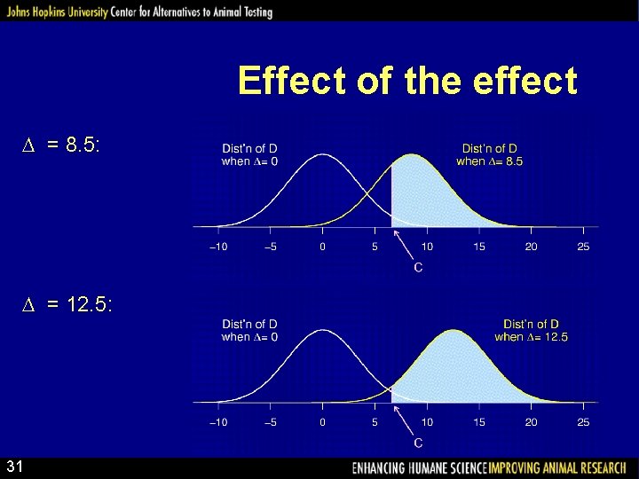
Effect of the effect = 8. 5: = 12. 5: 31

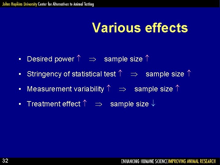
Various effects • Desired power sample size • Stringency of statistical test • Measurement variability • Treatment effect 32 sample size

Determining sample size The things you need to know: • • Structure of the experiment Method for analysis Chosen significance level, (usually 5%) Desired power (usually 80%) • Variability in the measurements – if necessary, perform a pilot study • The smallest meaningful effect 33

A formula d re o s n e C 34

Reducing sample size • Reduce the number of treatment groups being compared. • Find a more precise measurement (e. g. , average time to effect rather than proportion sick). • Decrease the variability in the measurements. – Make subjects more homogeneous. – Use stratification. – Control for other variables (e. g. , weight). – Average multiple measurements on each subject. 35

Final conclusions • Experiments should be designed. • Good design and good analysis can lead to reduced sample sizes. • Consult an expert on both the analysis and the design of your experiment. 36

Resources • ML Samuels, JA Witmer (2003) Statistics for the Life Sciences, 3 rd edition. Prentice Hall. – An excellent introductory text. • GW Oehlert (2000) A First Course in Design and Analysis of Experiments. WH Freeman & Co. – Includes a more advanced treatment of experimental design. • Course: Statistics for Laboratory Scientists (Biostatistics 140. 615 -616, Johns Hopkins Bloomberg Sch. Pub. Health) – Intoductory statistics course, intended for experimental scientists. – Greatly expands upon the topics presented here. 37