Experimental Design and Optimisation Rik Henson With thanks

Experimental Design and Optimisation Rik Henson With thanks to: Karl Friston, Oliver Josephs

Overview 1. A Taxonomy of Designs 2. Blocked vs Randomised Designs 3. Efficient Designs

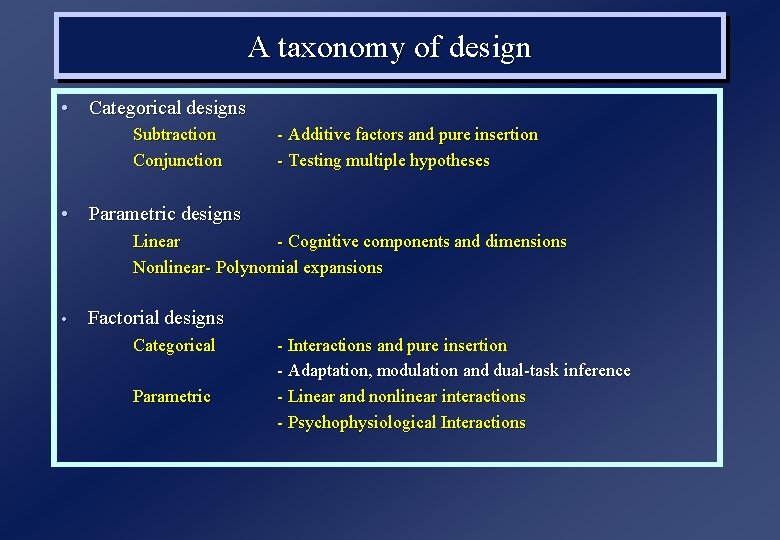
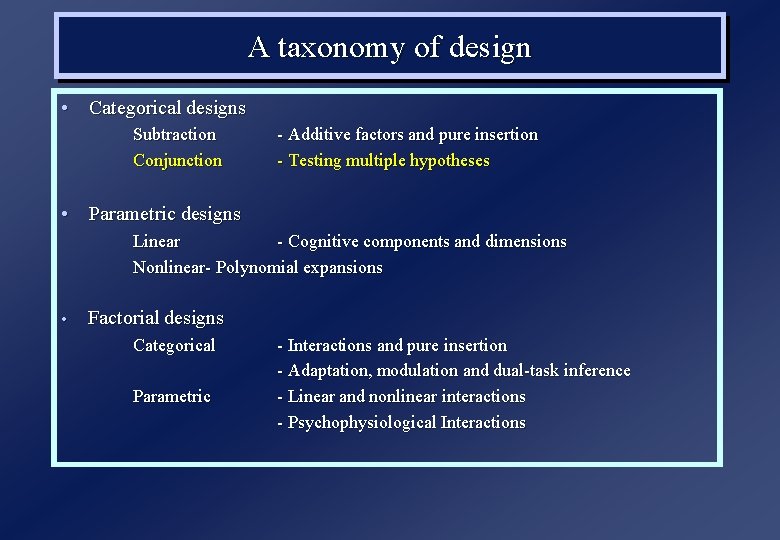
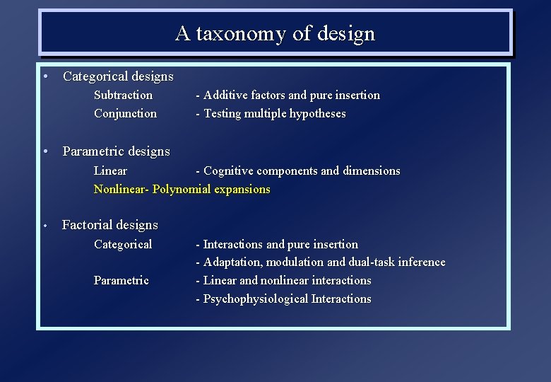
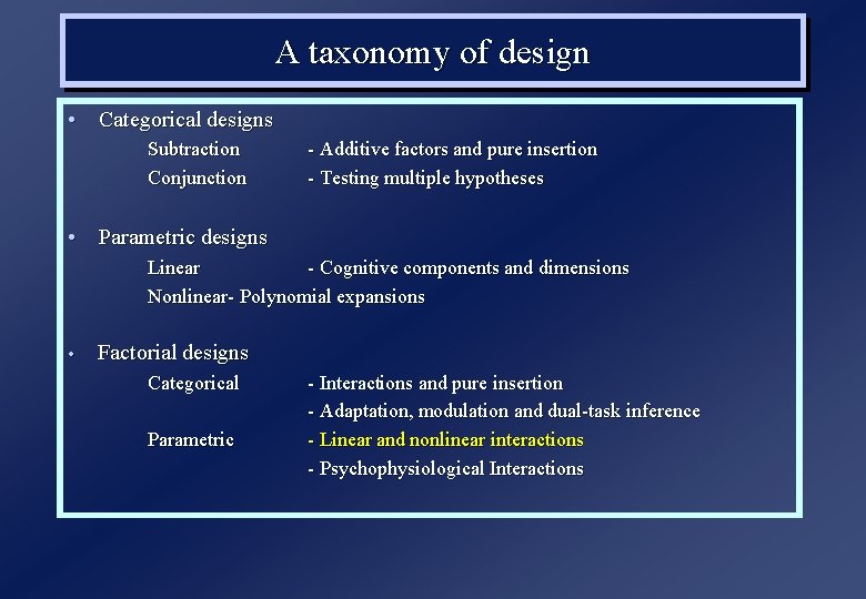
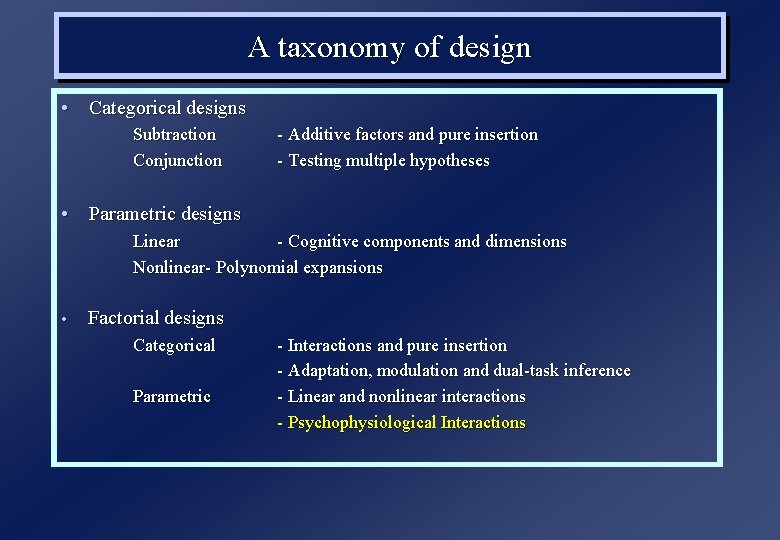
A taxonomy of design • Categorical designs Subtraction Conjunction - Additive factors and pure insertion - Testing multiple hypotheses • Parametric designs Linear - Cognitive components and dimensions Nonlinear- Polynomial expansions • Factorial designs Categorical Parametric - Interactions and pure insertion - Adaptation, modulation and dual-task inference - Linear and nonlinear interactions - Psychophysiological Interactions

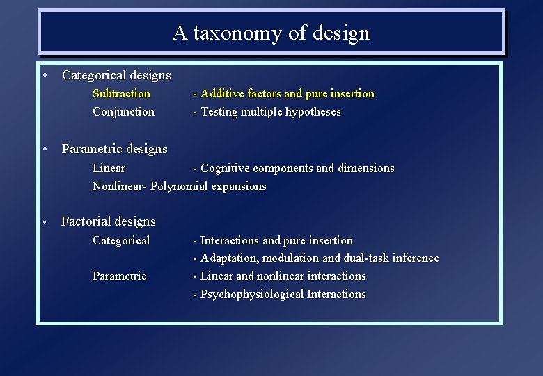
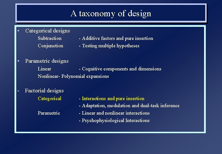
A taxonomy of design • Categorical designs Subtraction Conjunction - Additive factors and pure insertion - Testing multiple hypotheses • Parametric designs Linear - Cognitive components and dimensions Nonlinear- Polynomial expansions • Factorial designs Categorical Parametric - Interactions and pure insertion - Adaptation, modulation and dual-task inference - Linear and nonlinear interactions - Psychophysiological Interactions

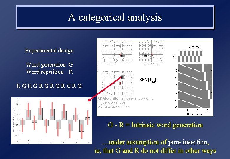
A categorical analysis Experimental design Word generation G Word repetition R RGRGRG G - R = Intrinsic word generation …under assumption of pure insertion, ie, that G and R do not differ in other ways

A taxonomy of design • Categorical designs Subtraction Conjunction - Additive factors and pure insertion - Testing multiple hypotheses • Parametric designs Linear - Cognitive components and dimensions Nonlinear- Polynomial expansions • Factorial designs Categorical Parametric - Interactions and pure insertion - Adaptation, modulation and dual-task inference - Linear and nonlinear interactions - Psychophysiological Interactions

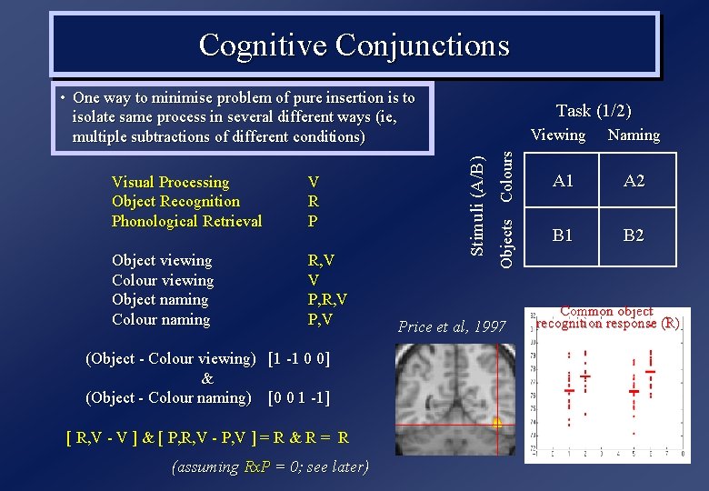
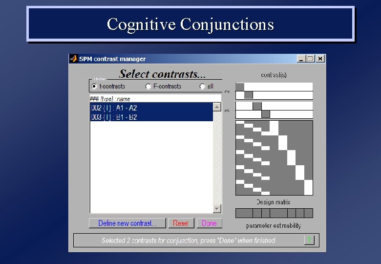
Cognitive Conjunctions • One way to minimise problem of pure insertion is to isolate same process in several different ways (ie, multiple subtractions of different conditions) Object viewing Colour viewing Object naming Colour naming R, V V P, R, V P, V (Object - Colour viewing) [1 -1 0 0] & (Object - Colour naming) [0 0 1 -1] [ R, V - V ] & [ P, R, V - P, V ] = R & R = R (assuming Rx. P = 0; see later) Objects Colours V R P Viewing Stimuli (A/B) Visual Processing Object Recognition Phonological Retrieval Task (1/2) Price et al, 1997 Naming A 1 A 2 B 1 B 2 Common object recognition response (R)

Cognitive Conjunctions

A taxonomy of design • Categorical designs Subtraction Conjunction - Additive factors and pure insertion - Testing multiple hypotheses • Parametric designs Linear - Cognitive components and dimensions Nonlinear- Polynomial expansions • Factorial designs Categorical Parametric - Interactions and pure insertion - Adaptation, modulation and dual-task inference - Linear and nonlinear interactions - Psychophysiological Interactions

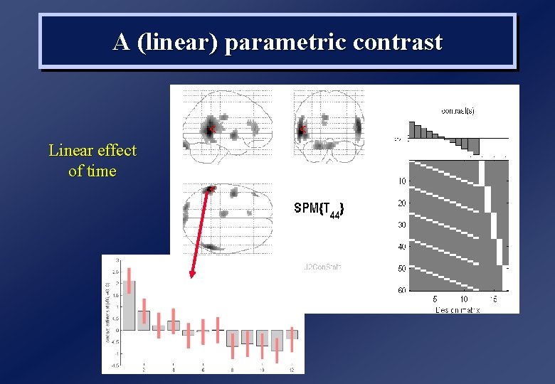
A (linear) parametric contrast Linear effect of time

A taxonomy of design • Categorical designs Subtraction Conjunction - Additive factors and pure insertion - Testing multiple hypotheses • Parametric designs Linear - Cognitive components and dimensions Nonlinear- Polynomial expansions • Factorial designs Categorical Parametric - Interactions and pure insertion - Adaptation, modulation and dual-task inference - Linear and nonlinear interactions - Psychophysiological Interactions

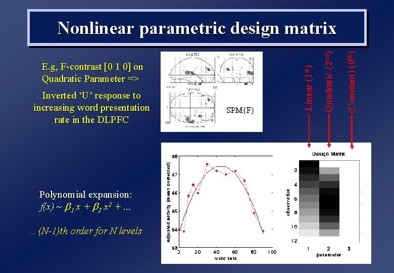
Polynomial expansion: f(x) ~ b 1 x + b 2 x 2 +. . . …(N-1)th order for N levels SPM{F} (Constant) (0 th) Inverted ‘U’ response to increasing word presentation rate in the DLPFC Quadratic (2 nd) E. g, F-contrast [0 1 0] on Quadratic Parameter => Linear (1 st) Nonlinear parametric design matrix

A taxonomy of design • Categorical designs Subtraction Conjunction - Additive factors and pure insertion - Testing multiple hypotheses • Parametric designs Linear - Cognitive components and dimensions Nonlinear- Polynomial expansions • Factorial designs Categorical Parametric - Interactions and pure insertion - Adaptation, modulation and dual-task inference - Linear and nonlinear interactions - Psychophysiological Interactions

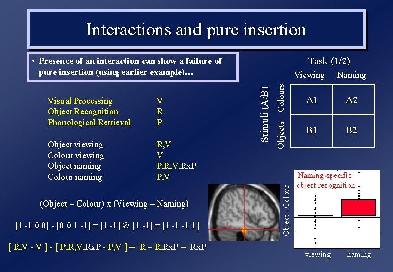
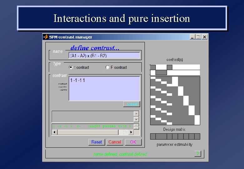
Interactions and pure insertion Task (1/2) • Presence of an interaction can show a failure of pure insertion (using earlier example)… R, V V P, R, V, Rx. P P, V (Object – Colour) x (Viewing – Naming) [1 -1 0 0] - [0 0 1 -1] = [1 -1 -1 1] [ R, V - V ] - [ P, R, V, Rx. P - P, V ] = R – R, Rx. P = Rx. P Objects Colours Object viewing Colour viewing Object naming Colour naming Object - Colour V R P Stimuli (A/B) Visual Processing Object Recognition Phonological Retrieval Viewing Naming A 1 A 2 B 1 B 2 Naming-specific object recognition viewing naming

Interactions and pure insertion

A taxonomy of design • Categorical designs Subtraction Conjunction - Additive factors and pure insertion - Testing multiple hypotheses • Parametric designs Linear - Cognitive components and dimensions Nonlinear- Polynomial expansions • Factorial designs Categorical Parametric - Interactions and pure insertion - Adaptation, modulation and dual-task inference - Linear and nonlinear interactions - Psychophysiological Interactions

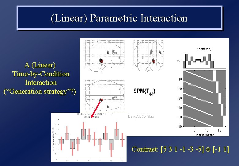
(Linear) Parametric Interaction A (Linear) Time-by-Condition Interaction (“Generation strategy”? ) Contrast: [5 3 1 -1 -3 -5] [-1 1]

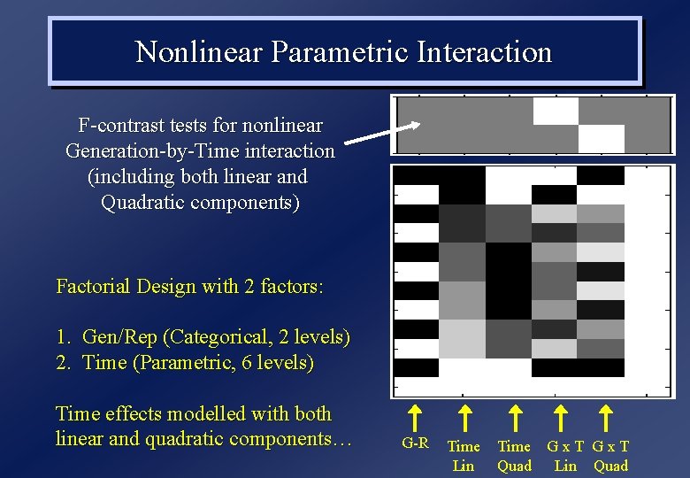
Nonlinear Parametric Interaction F-contrast tests for nonlinear Generation-by-Time interaction (including both linear and Quadratic components) Factorial Design with 2 factors: 1. Gen/Rep (Categorical, 2 levels) 2. Time (Parametric, 6 levels) Time effects modelled with both linear and quadratic components… G-R Time Lin Time G x T Quad Lin Quad

A taxonomy of design • Categorical designs Subtraction Conjunction - Additive factors and pure insertion - Testing multiple hypotheses • Parametric designs Linear - Cognitive components and dimensions Nonlinear- Polynomial expansions • Factorial designs Categorical Parametric - Interactions and pure insertion - Adaptation, modulation and dual-task inference - Linear and nonlinear interactions - Psychophysiological Interactions

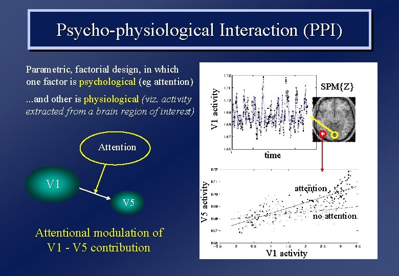
Psycho-physiological Interaction (PPI) Parametric, factorial design, in which one factor is psychological (eg attention) V 1 activity . . . and other is physiological (viz. activity extracted from a brain region of interest) Attention V 5 Attentional modulation of V 1 - V 5 contribution time V 5 activity V 1 SPM{Z} attention no attention V 1 activity

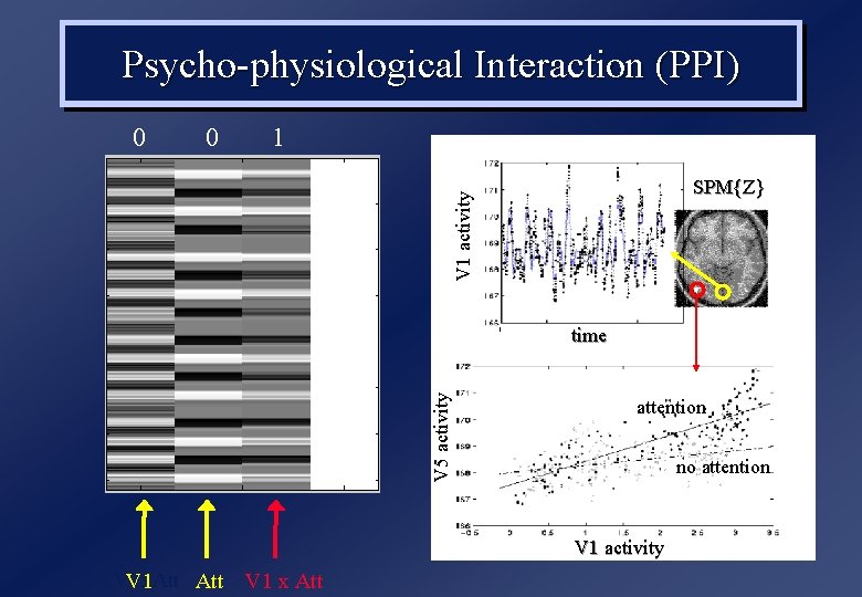
Psycho-physiological Interaction (PPI) 0 1 SPM{Z} V 1 activity 0 V 5 activity time attention no attention V 1 activity V 1 x. Att V 1 x Att

Overview 1. A Taxonomy of Designs 2. Blocked vs Randomised Designs 3. Efficient Designs

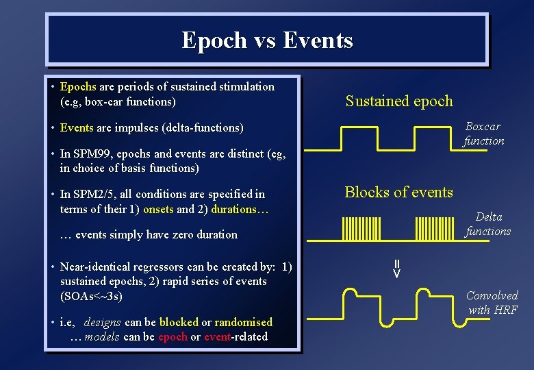
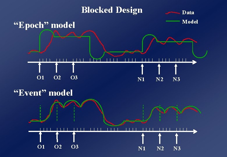
Epoch vs Events • Epochs are periods of sustained stimulation (e. g, box-car functions) Sustained epoch Boxcar function • Events are impulses (delta-functions) • In SPM 99, epochs and events are distinct (eg, in choice of basis functions) • In SPM 2/5, all conditions are specified in terms of their 1) onsets and 2) durations… Blocks of events Delta functions … events simply have zero duration • i. e, designs can be blocked or randomised … models can be epoch or event-related => • Near-identical regressors can be created by: 1) sustained epochs, 2) rapid series of events (SOAs<~3 s) Convolved with HRF

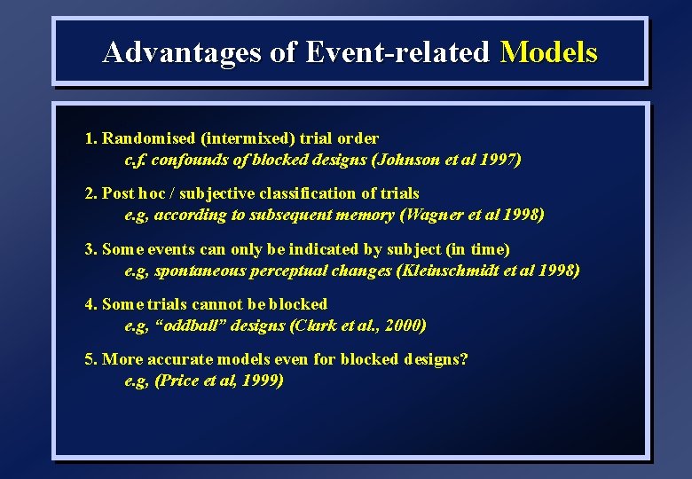
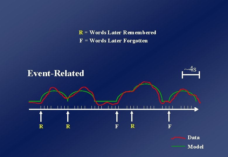
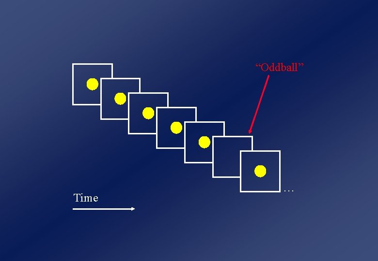
Advantages of Event-related Models 1. Randomised (intermixed) trial order c. f. confounds of blocked designs (Johnson et al 1997) 2. Post hoc / subjective classification of trials e. g, according to subsequent memory (Wagner et al 1998) 3. Some events can only be indicated by subject (in time) e. g, spontaneous perceptual changes (Kleinschmidt et al 1998) 4. Some trials cannot be blocked e. g, “oddball” designs (Clark et al. , 2000) 5. More accurate models even for blocked designs? e. g, (Price et al, 1999)

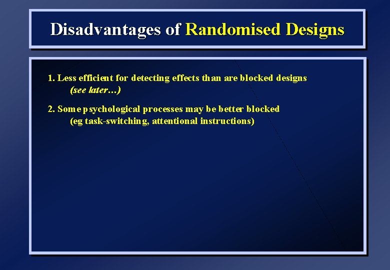
Disadvantages of Randomised Designs 1. Less efficient for detecting effects than are blocked designs (see later…) 2. Some psychological processes may be better blocked (eg task-switching, attentional instructions)

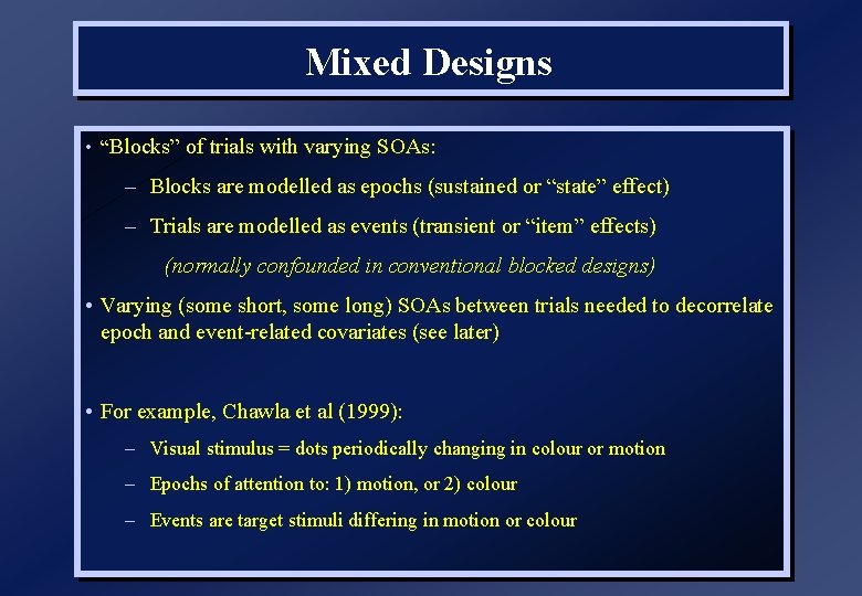
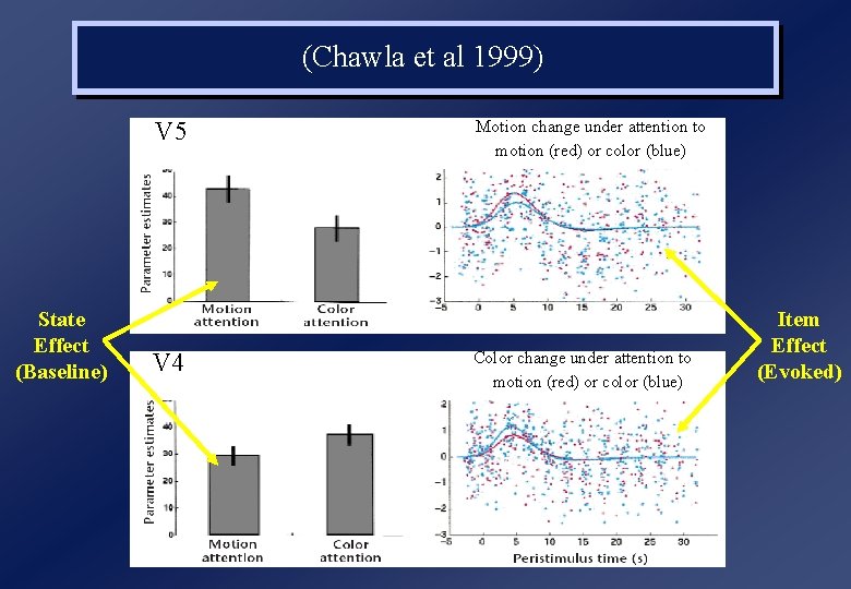
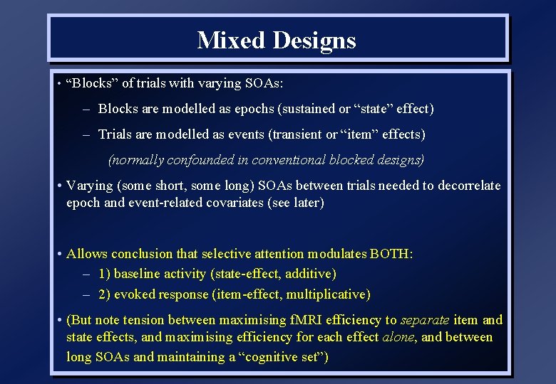
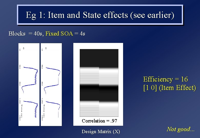
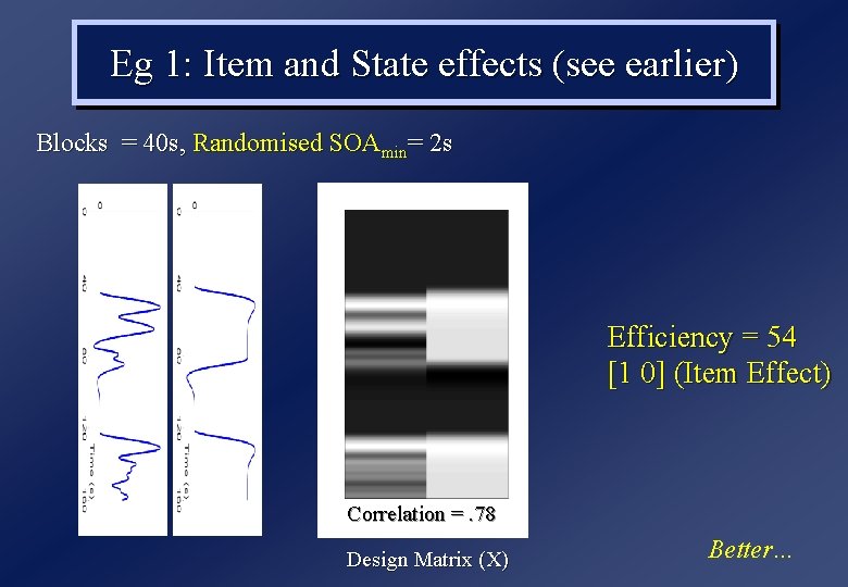
Mixed Designs • “Blocks” of trials with varying SOAs: – Blocks are modelled as epochs (sustained or “state” effect) – Trials are modelled as events (transient or “item” effects) (normally confounded in conventional blocked designs) • Varying (some short, some long) SOAs between trials needed to decorrelate epoch and event-related covariates (see later) • For example, Chawla et al (1999): – Visual stimulus = dots periodically changing in colour or motion – Epochs of attention to: 1) motion, or 2) colour – Events are target stimuli differing in motion or colour

(Chawla et al 1999) V 5 State Effect (Baseline) V 4 Motion change under attention to motion (red) or color (blue) Color change under attention to motion (red) or color (blue) Item Effect (Evoked)

Mixed Designs • “Blocks” of trials with varying SOAs: – Blocks are modelled as epochs (sustained or “state” effect) – Trials are modelled as events (transient or “item” effects) (normally confounded in conventional blocked designs) • Varying (some short, some long) SOAs between trials needed to decorrelate epoch and event-related covariates (see later) • Allows conclusion that selective attention modulates BOTH: – 1) baseline activity (state-effect, additive) – 2) evoked response (item-effect, multiplicative) • (But note tension between maximising f. MRI efficiency to separate item and state effects, and maximising efficiency for each effect alone, and between long SOAs and maintaining a “cognitive set”)

Overview 1. A Taxonomy of Designs 2. Blocked vs Randomised Designs 3. Efficient Designs

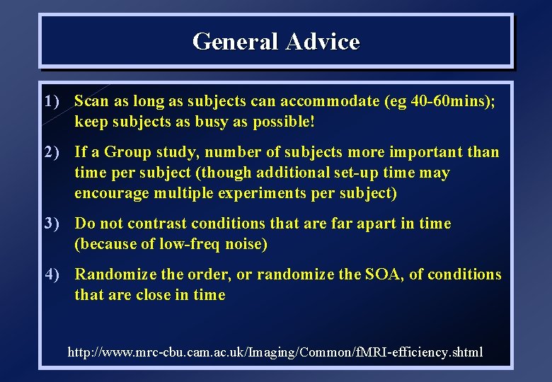
General Advice 1) Scan as long as subjects can accommodate (eg 40 -60 mins); keep subjects as busy as possible! 2) If a Group study, number of subjects more important than time per subject (though additional set-up time may encourage multiple experiments per subject) 3) Do not contrast conditions that are far apart in time (because of low-freq noise) 4) Randomize the order, or randomize the SOA, of conditions that are close in time http: //www. mrc-cbu. cam. ac. uk/Imaging/Common/f. MRI-efficiency. shtml

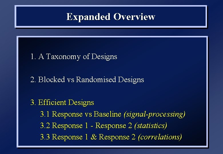
Expanded Overview 1. A Taxonomy of Designs 2. Blocked vs Randomised Designs 3. Efficient Designs 3. 1 Response vs Baseline (signal-processing) 3. 2 Response 1 - Response 2 (statistics) 3. 3 Response 1 & Response 2 (correlations)

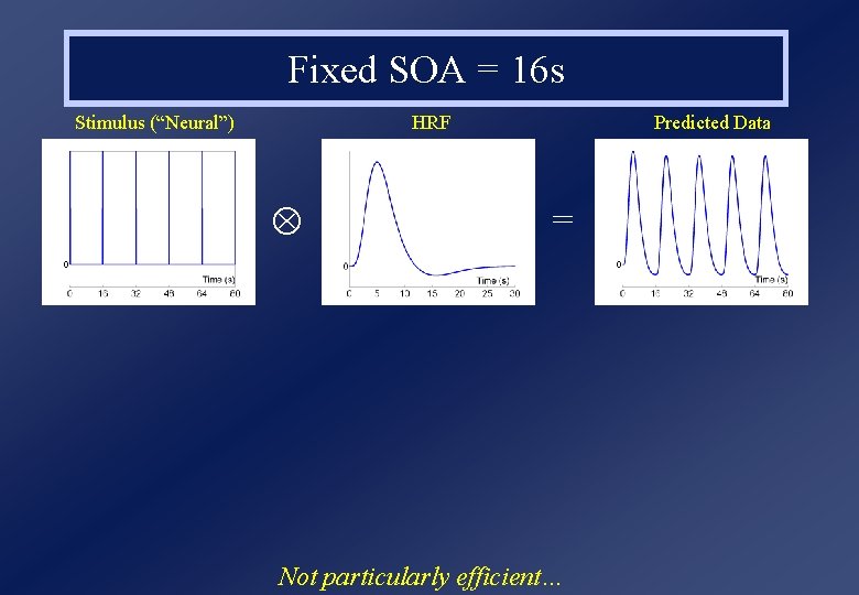
Fixed SOA = 16 s Stimulus (“Neural”) HRF Predicted Data = Not particularly efficient…

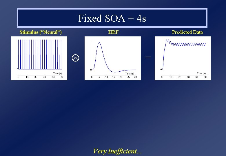
Fixed SOA = 4 s Stimulus (“Neural”) HRF Predicted Data = Very Inefficient…

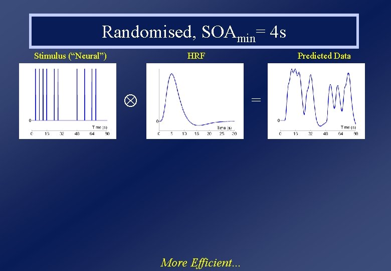
Randomised, SOAmin= 4 s Stimulus (“Neural”) HRF Predicted Data = More Efficient…

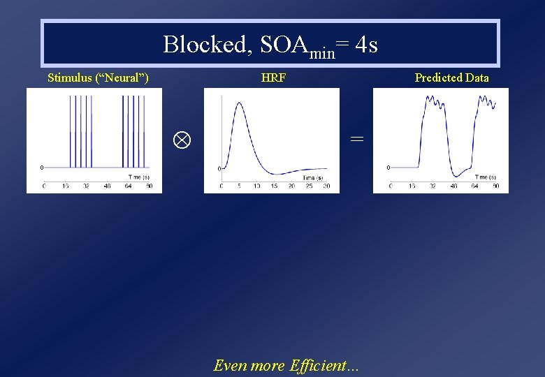
Blocked, SOAmin= 4 s Stimulus (“Neural”) HRF Predicted Data = Even more Efficient…

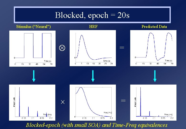
Blocked, epoch = 20 s Stimulus (“Neural”) HRF Predicted Data = = Blocked-epoch (with small SOA) and Time-Freq equivalences

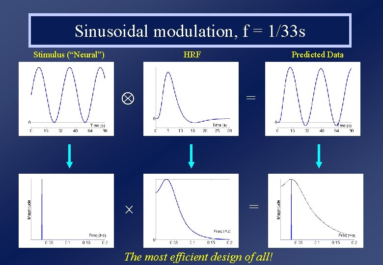
Sinusoidal modulation, f = 1/33 s Stimulus (“Neural”) HRF Predicted Data = = The most efficient design of all!

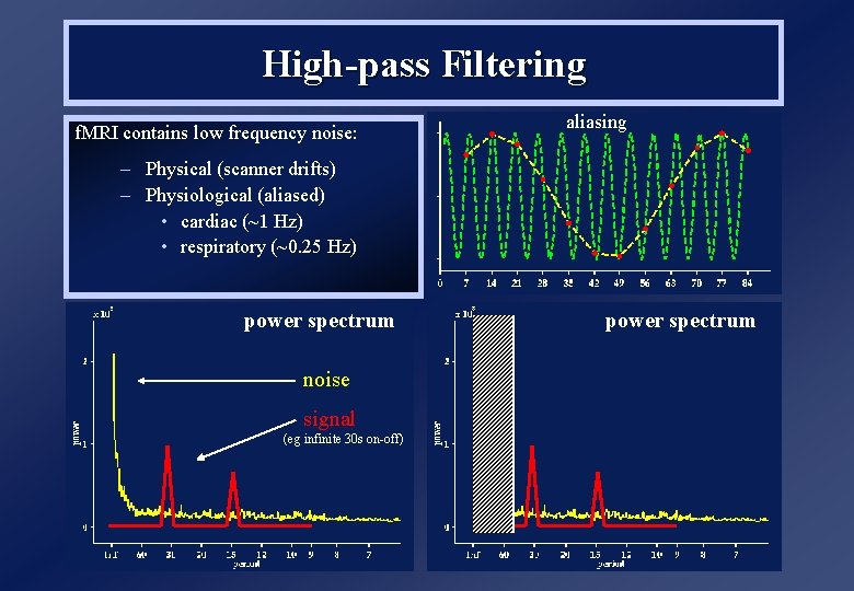
High-pass Filtering f. MRI contains low frequency noise: aliasing – Physical (scanner drifts) – Physiological (aliased) • cardiac (~1 Hz) • respiratory (~0. 25 Hz) power spectrum noise signal (eg infinite 30 s on-off) power spectrum highpass filter

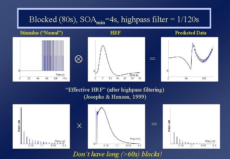
Blocked (80 s), SOAmin=4 s, highpass filter = 1/120 s Stimulus (“Neural”) HRF Predicted Data = “Effective HRF” (after highpass filtering) (Josephs & Henson, 1999) = Don’t have long (>60 s) blocks!

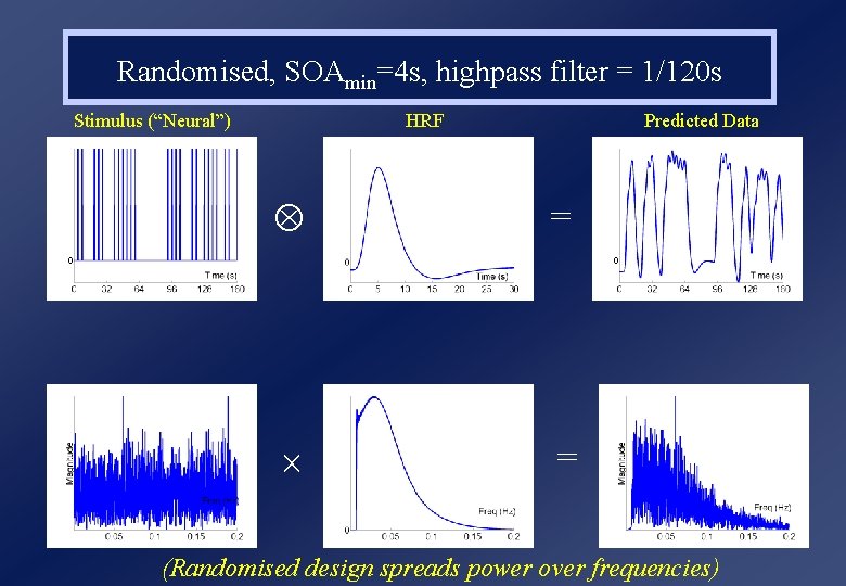
Randomised, SOAmin=4 s, highpass filter = 1/120 s Stimulus (“Neural”) HRF Predicted Data = = (Randomised design spreads power over frequencies)

2. How about multiple conditions? • We have talked about detecting a basic response vs baseline, but how about detecting differences between two or more response-types (event-types)?

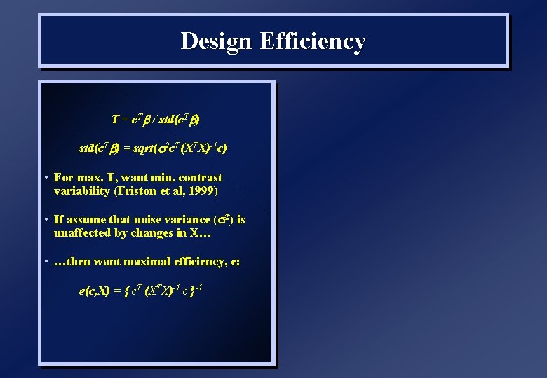
Design Efficiency T = c. Tb / std(c. Tb) = sqrt( 2 c. T(XTX)-1 c) • For max. T, want min. contrast variability (Friston et al, 1999) • If assume that noise variance ( 2) is unaffected by changes in X… • …then want maximal efficiency, e: e(c, X) = { c. T (XTX)-1 c }-1

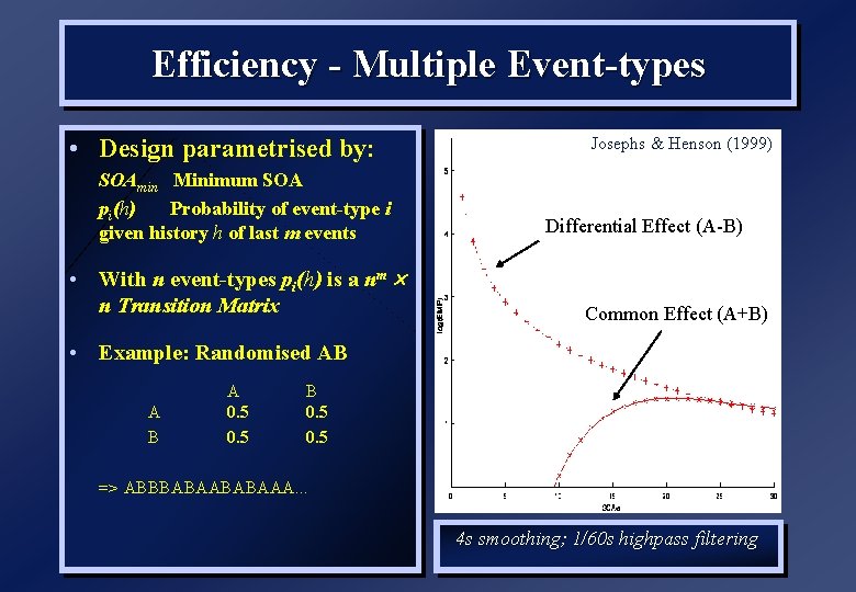
Efficiency - Multiple Event-types • Design parametrised by: SOAmin Minimum SOA pi(h) Probability of event-type i given history h of last m events • With n event-types pi(h) is a nm n Transition Matrix Josephs & Henson (1999) Differential Effect (A-B) Common Effect (A+B) • Example: Randomised AB A 0. 5 B 0. 5 => ABBBABAAA. . . 4 s smoothing; 1/60 s highpass filtering

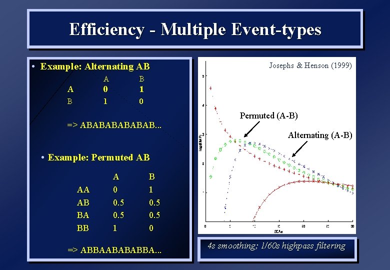
Efficiency - Multiple Event-types • Example: Alternating AB A 0 1 B 1 0 => ABABAB. . . Josephs & Henson (1999) Permuted (A-B) Alternating (A-B) • Example: Permuted AB AA AB BA BB A 0 0. 5 1 B 1 0. 5 0 => ABBAABABABBA. . . 4 s smoothing; 1/60 s highpass filtering

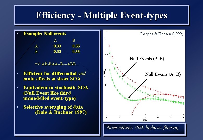
Efficiency - Multiple Event-types • Example: Null events A B A 0. 33 Josephs & Henson (1999) B 0. 33 => AB-BAA--B---ABB. . . • Efficient for differential and main effects at short SOA Null Events (A-B) Null Events (A+B) • Equivalent to stochastic SOA (Null Event like third unmodelled event-type) • Selective averaging of data (Dale & Buckner 1997) 4 s smoothing; 1/60 s highpass filtering

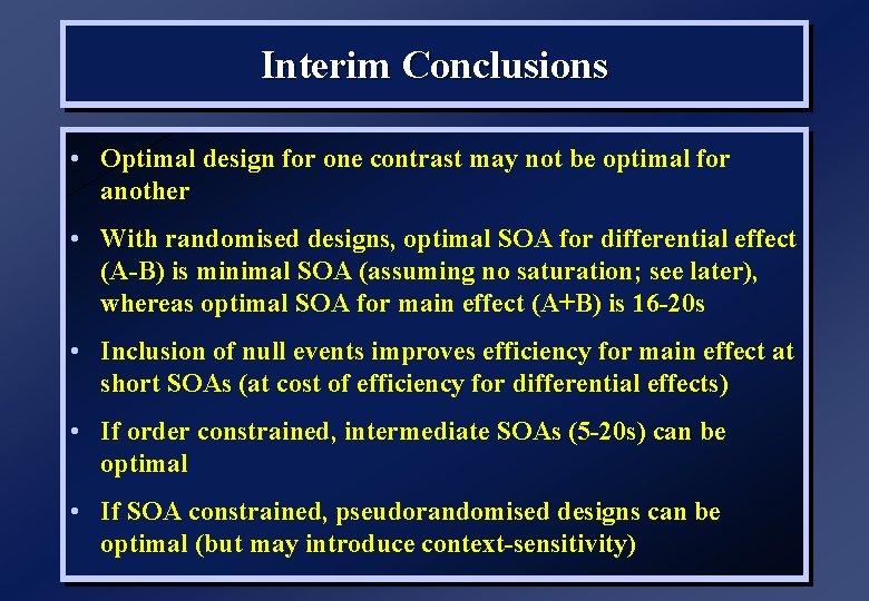
Interim Conclusions • Optimal design for one contrast may not be optimal for another • With randomised designs, optimal SOA for differential effect (A-B) is minimal SOA (assuming no saturation; see later), whereas optimal SOA for main effect (A+B) is 16 -20 s • Inclusion of null events improves efficiency for main effect at short SOAs (at cost of efficiency for differential effects) • If order constrained, intermediate SOAs (5 -20 s) can be optimal • If SOA constrained, pseudorandomised designs can be optimal (but may introduce context-sensitivity)

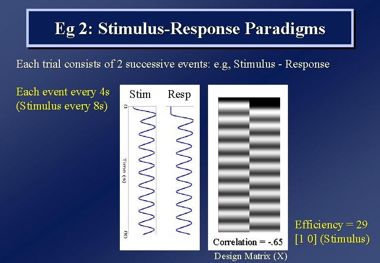
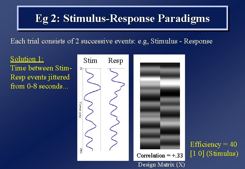
3. How about separating responses? What if interested in both contrasts [1 0] and [0 1]? • For example: 1) Mixed designs (item-state effects) 2) Working Memory trials (stimulus-response) • In the efficiency of a contrast (see earlier): e(c, X) = { c. T (XTX)-1 c }-1 XTX represents covariance of regressors in design matrix • High covariance increases elements of (XTX)-1 • So, when correlation between regressors, efficiency to detect effect of each one separately is reduced

Correlations between Regressors [1 -1] [1 1] Negative correlation between two regressors means separate (orthogonal) effect of each is estimated poorly, though difference between regressors estimated well

Eg 1: Item and State effects (see earlier) Blocks = 40 s, Fixed SOA = 4 s Efficiency = 16 [1 0] (Item Effect) Correlation =. 97 Design Matrix (X) Not good…

Eg 1: Item and State effects (see earlier) Blocks = 40 s, Randomised SOAmin= 2 s Efficiency = 54 [1 0] (Item Effect) Correlation =. 78 Design Matrix (X) Better…

Eg 2: Stimulus-Response Paradigms Each trial consists of 2 successive events: e. g, Stimulus - Response Each event every 4 s (Stimulus every 8 s) Stim Resp Efficiency = 29 Correlation = -. 65 [1 0] (Stimulus) Design Matrix (X)

Eg 2: Stimulus-Response Paradigms Each trial consists of 2 successive events: e. g, Stimulus - Response Solution 1: Time between Stim. Resp events jittered from 0 -8 seconds. . . Stim Resp Efficiency = 40 Correlation = +. 33 [1 0] (Stimulus) Design Matrix (X)

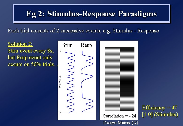
Eg 2: Stimulus-Response Paradigms Each trial consists of 2 successive events: e. g, Stimulus - Response Solution 2: Stim event every 8 s, but Resp event only occurs on 50% trials. . . Resp Efficiency = 47 Correlation = -. 24 [1 0] (Stimulus) Design Matrix (X)

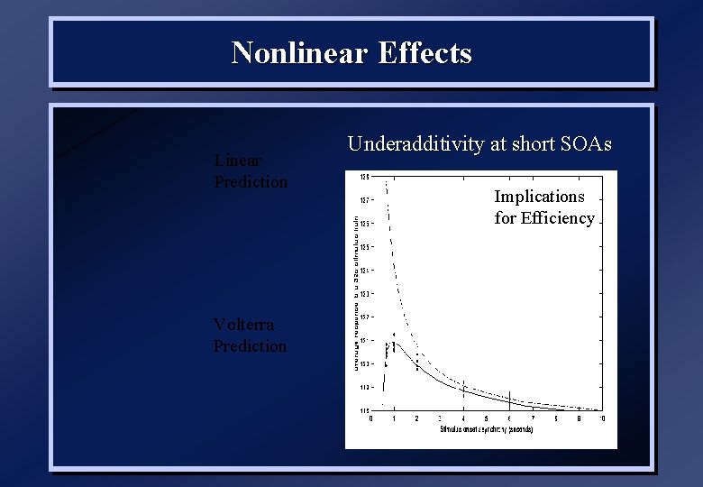
Nonlinear Effects Linear Prediction Volterra Prediction Underadditivity at short SOAs Implications for Efficiency

The End This talk appears as Chapter 15 in the SPM book: http: //www. mrc-cbu. cam. ac. uk/~rh 01/Henson_Design_SPMBook_2006_preprint. pdf For further info on how to design an efficient f. MRI experiment, see: http: //www. mrc-cbu. cam. ac. uk/Imaging/Common/f. MRI-efficiency. shtml

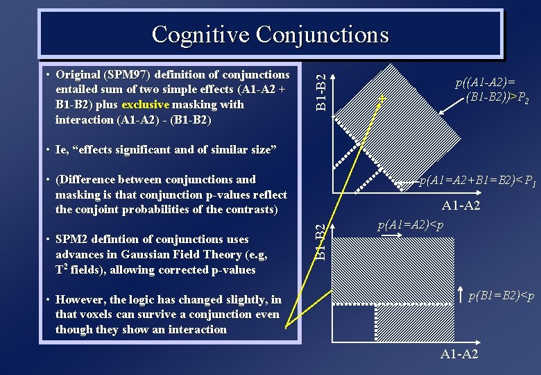
• Original (SPM 97) definition of conjunctions entailed sum of two simple effects (A 1 -A 2 + B 1 -B 2) plus exclusive masking with interaction (A 1 -A 2) - (B 1 -B 2) B 1 -B 2 Cognitive Conjunctions p((A 1 -A 2)= (B 1 -B 2))>P 2 + • Ie, “effects significant and of similar size” • (Difference between conjunctions and masking is that conjunction p-values reflect the conjoint probabilities of the contrasts) • However, the logic has changed slightly, in that voxels can survive a conjunction even though they show an interaction A 1 -A 2 B 1 -B 2 • SPM 2 defintion of conjunctions uses advances in Gaussian Field Theory (e. g, T 2 fields), allowing corrected p-values p(A 1=A 2+B 1=B 2)<P 1 p(A 1=A 2)<p + p(B 1=B 2)<p A 1 -A 2

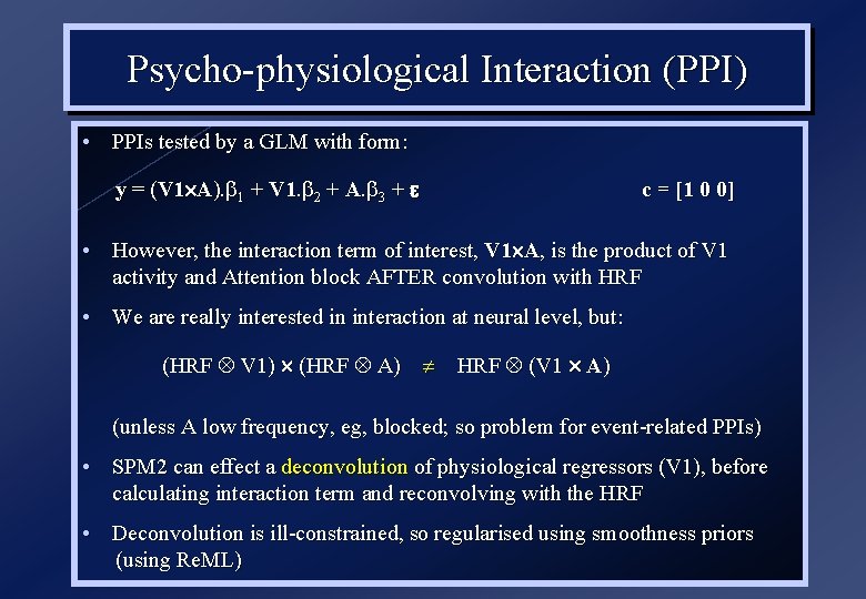
Psycho-physiological Interaction (PPI) • PPIs tested by a GLM with form: y = (V 1 A). b 1 + V 1. b 2 + A. b 3 + e c = [1 0 0] • However, the interaction term of interest, V 1 A, is the product of V 1 activity and Attention block AFTER convolution with HRF • We are really interested in interaction at neural level, but: (HRF V 1) (HRF A) HRF (V 1 A) (unless A low frequency, eg, blocked; so problem for event-related PPIs) • SPM 2 can effect a deconvolution of physiological regressors (V 1), before calculating interaction term and reconvolving with the HRF • Deconvolution is ill-constrained, so regularised using smoothness priors (using Re. ML)

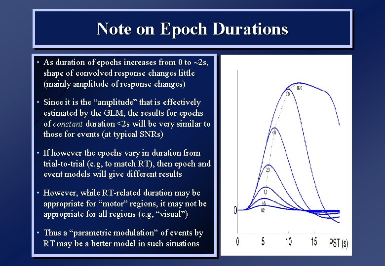
Note on Epoch Durations • As duration of epochs increases from 0 to ~2 s, shape of convolved response changes little (mainly amplitude of response changes) • Since it is the “amplitude” that is effectively estimated by the GLM, the results for epochs of constant duration <2 s will be very similar to those for events (at typical SNRs) • If however the epochs vary in duration from trial-to-trial (e. g, to match RT), then epoch and event models will give different results • However, while RT-related duration may be appropriate for “motor” regions, it may not be appropriate for all regions (e. g, “visual”) • Thus a “parametric modulation” of events by RT may be a better model in such situations

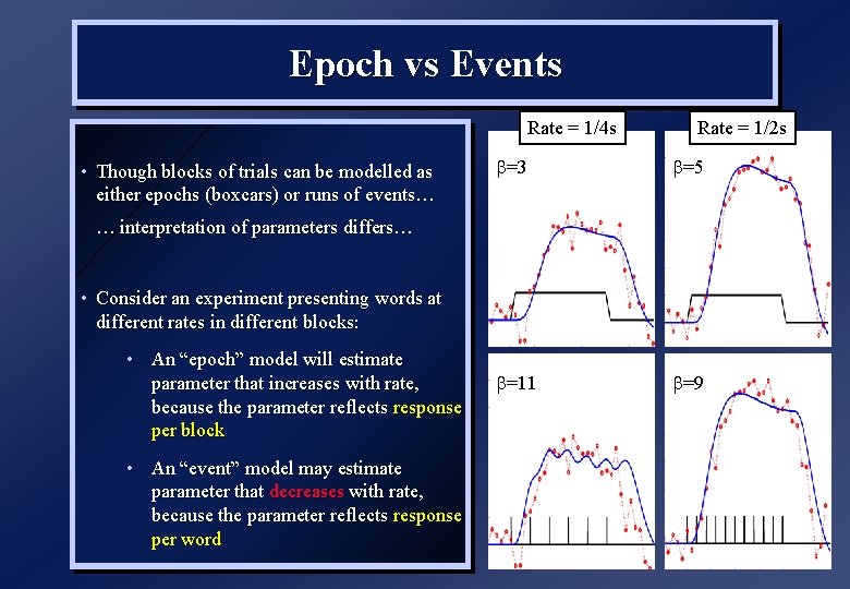
Epoch vs Events Rate = 1/4 s • Though blocks of trials can be modelled as either epochs (boxcars) or runs of events… Rate = 1/2 s b=3 b=5 b=11 b=9 … interpretation of parameters differs… • Consider an experiment presenting words at different rates in different blocks: • An “epoch” model will estimate parameter that increases with rate, because the parameter reflects response per block • An “event” model may estimate parameter that decreases with rate, because the parameter reflects response per word

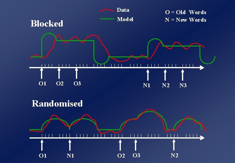
Data Model Blocked O 1 O 2 O = Old Words N = New Words O 3 N 1 N 2 N 3 Randomised O 1 N 1 O 2 O 3 N 2

R = Words Later Remembered F = Words Later Forgotten ~4 s Event-Related R R F Data Model

“Oddball” Time …

Blocked Design Data Model “Epoch” model O 1 O 2 O 3 N 1 N 2 N 3 “Event” model O 1 O 2 O 3

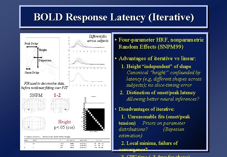
BOLD Response Latency (Iterative) Different fits across subjects Peak Delay Height • Advantages of iterative vs linear: Dispersion Onset Delay FIR used to deconvolve data, before nonlinear fitting over PST SNPM • Four-parameter HRF, nonparametric Random Effects (SNPM 99) 1 -2 Height p<. 05 (cor) 1. Height “independent” of shape Canonical “height” confounded by latency (e. g, different shapes across subjects); no slice-timing error 2. Distinction of onset/peak latency Allowing better neural inferences? • Disadvantages of iterative: 1. Unreasonable fits (onset/peak tension) Priors on parameter distributions? (Bayesian estimation) 2. Local minima, failure of convergence?

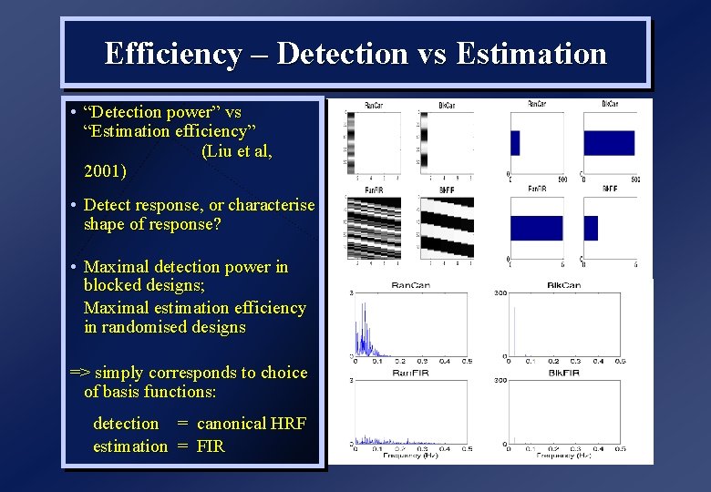
Efficiency – Detection vs Estimation • “Detection power” vs “Estimation efficiency” (Liu et al, 2001) • Detect response, or characterise shape of response? • Maximal detection power in blocked designs; Maximal estimation efficiency in randomised designs => simply corresponds to choice of basis functions: detection = canonical HRF estimation = FIR

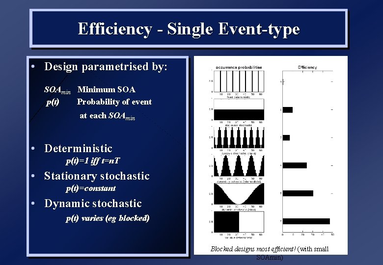
Efficiency - Single Event-type • Design parametrised by: SOAmin Minimum SOA p(t) Probability of event at each SOAmin • Deterministic p(t)=1 iff t=n. T • Stationary stochastic p(t)=constant • Dynamic stochastic p(t) varies (eg blocked) Blocked designs most efficient! (with small SOAmin)

1. Basic Response vs Baseline To detect a basic event-related response versus baseline… • Do not present stimuli at a fixed rate • Varying the SOA (eg via null events), with a minimal shortest SOA, is more efficient • Presenting stimuli rapidly within on/off blocks of ~20 s is even more efficient (though psychological downsides, eg predictability? ) • Longer blocks (>60 seconds) can be confounded by lowfrequency noise