Experimental Analysis of Algorithms What to Measure Catherine

Experimental Analysis of Algorithms: What to Measure Catherine C. Mc. Geoch Amherst College

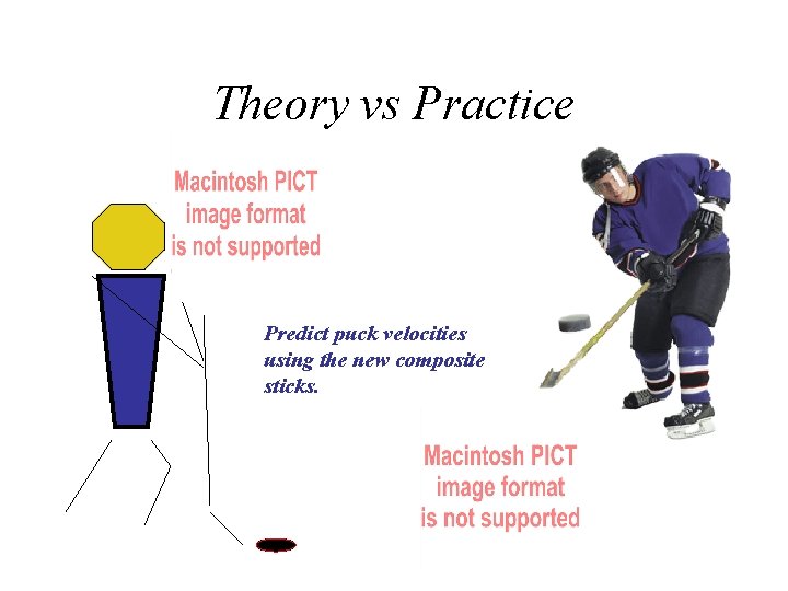
Theory vs Practice Predict puck velocities using the new composite sticks.

Isolate Components Control Factors Attach Probes

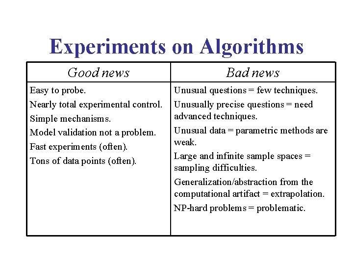
Experiments on Algorithms Good news Bad news Easy to probe. Nearly total experimental control. Simple mechanisms. Model validation not a problem. Fast experiments (often). Tons of data points (often). Unusual questions = few techniques. Unusually precise questions = need advanced techniques. Unusual data = parametric methods are weak. Large and infinite sample spaces = sampling difficulties. Generalization/abstraction from the computational artifact = extrapolation. NP-hard problems = problematic.

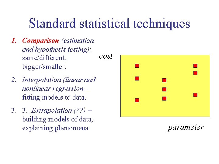
Standard statistical techniques 1. Comparison (estimation and hypothesis testing): cost same/different, bigger/smaller. 2. Interpolation (linear and nonlinear regression -fitting models to data. 3. 3. Extrapolation (? ? ) -building models of data, explaining phenomena. parameter

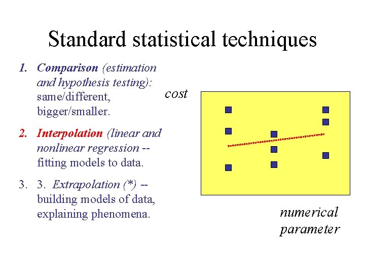
Standard statistical techniques 1. Comparison (estimation and hypothesis testing): cost same/different, bigger/smaller. 2. Interpolation (linear and nonlinear regression -fitting models to data. 3. 3. Extrapolation (*) -building models of data, explaining phenomena. numerical parameter

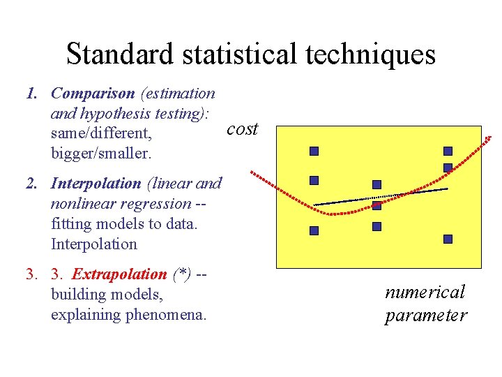
Standard statistical techniques 1. Comparison (estimation and hypothesis testing): cost same/different, bigger/smaller. 2. Interpolation (linear and nonlinear regression -fitting models to data. Interpolation 3. 3. Extrapolation (*) -building models, explaining phenomena. numerical parameter

Some Nonstandard Techniques 1. Graphical analysis (GA) -- big data sets, unusual questions, interpolation, extrapolation. 2. Exploratory data analysis (EDA) -- model building, unusual data sets. 3. Variance reduction techniques -- simple mechanisms, complete control. 4. Biased estimators -- NP-Hard problems, large sample spaces. Today!

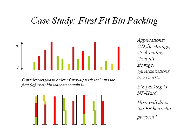
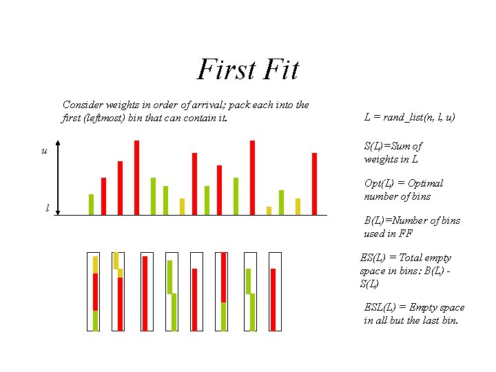
Case Study: First Fit Bin Packing u l Consider weights in order of arrival; pack each into the first (leftmost) bin that can contain it. Applications: CD file storage; stock cutting; i. Pod file storage; generalizations to 2 D, 3 D. . . Bin packing is NP-Hard. How well does the FF heuristic perform?

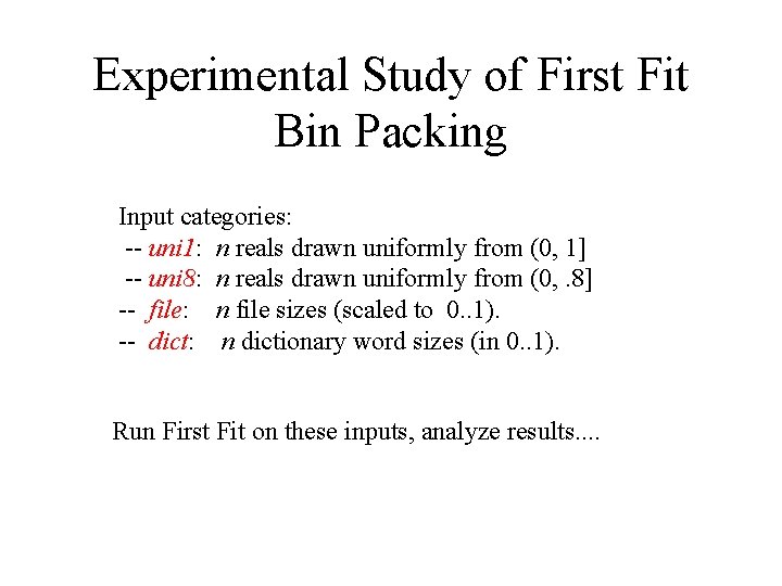
Experimental Study of First Fit Bin Packing Input categories: -- uni 1: n reals drawn uniformly from (0, 1] -- uni 8: n reals drawn uniformly from (0, . 8] -- file: n file sizes (scaled to 0. . 1). -- dict: n dictionary word sizes (in 0. . 1). Run First Fit on these inputs, analyze results. .

What to Measure? What performance indicator to use for assessing heuristic solution quality? The obvious choice: Number of Bins Other performance indicators suggested by data analysis: - Graphical analysis (GA) - Exploratory data analysis (EDA) - Variance reduction techniques (VRT) - Biased estimators Today’s topic!

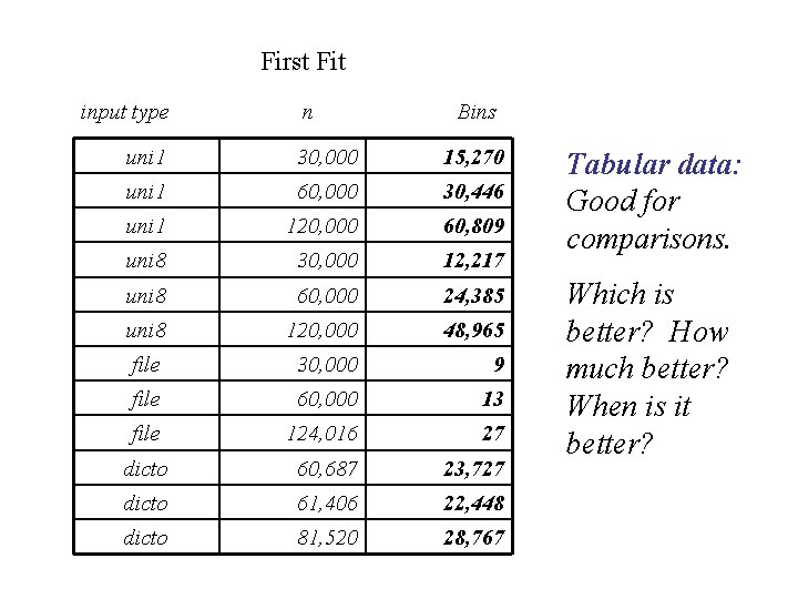
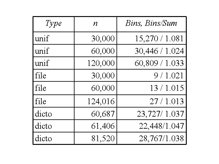
First Fit input type n Bins uni 1 30, 000 15, 270 uni 1 60, 000 30, 446 uni 1 120, 000 60, 809 uni 8 30, 000 12, 217 uni 8 60, 000 24, 385 uni 8 120, 000 48, 965 file 30, 000 9 file 60, 000 13 file 124, 016 27 dicto 60, 687 23, 727 dicto 61, 406 22, 448 dicto 81, 520 28, 767 Tabular data: Good for comparisons. Which is better? How much better? When is it better?

Graphical Analysis Identify trends Find common scales Discover anomalies Build models/explanations

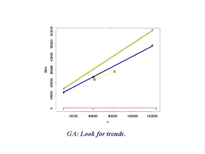
Graphical analysis: Locate Correlations GA: Look for trends.

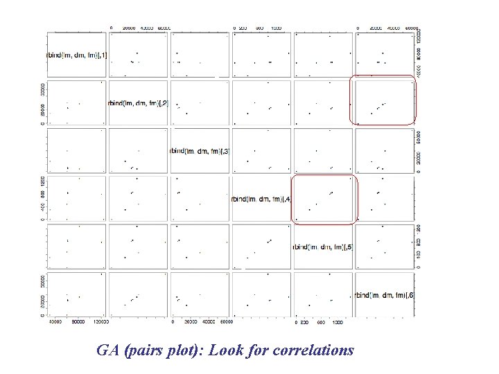
GA (pairs plot): Look for correlations

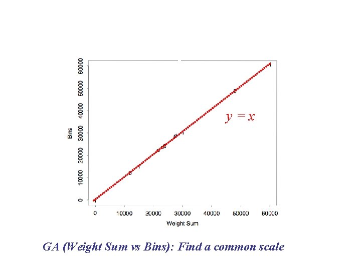
y=x GA (Weight Sum vs Bins): Find a common scale

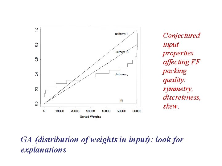
Conjectured input properties affecting FF packing quality: symmetry, discreteness, skew. GA (distribution of weights in input): look for explanations

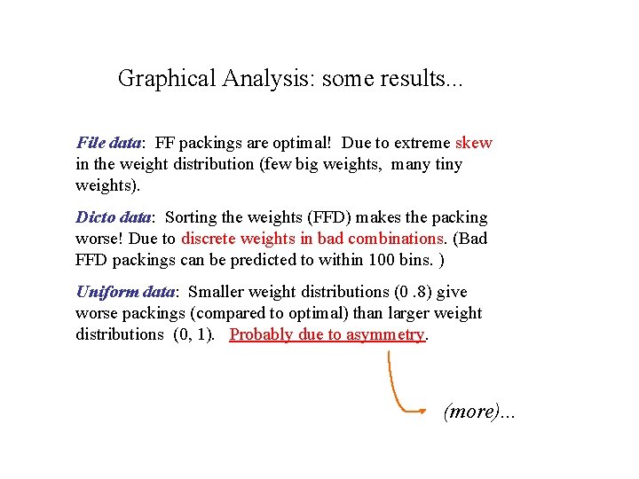
Graphical Analysis: some results. . . File data: FF packings are optimal! Due to extreme skew in the weight distribution (few big weights, many tiny weights). Dicto data: Sorting the weights (FFD) makes the packing worse! Due to discrete weights in bad combinations. (Bad FFD packings can be predicted to within 100 bins. ) Uniform data: Smaller weight distributions (0. 8) give worse packings (compared to optimal) than larger weight distributions (0, 1). Probably due to asymmetry. (more). . .

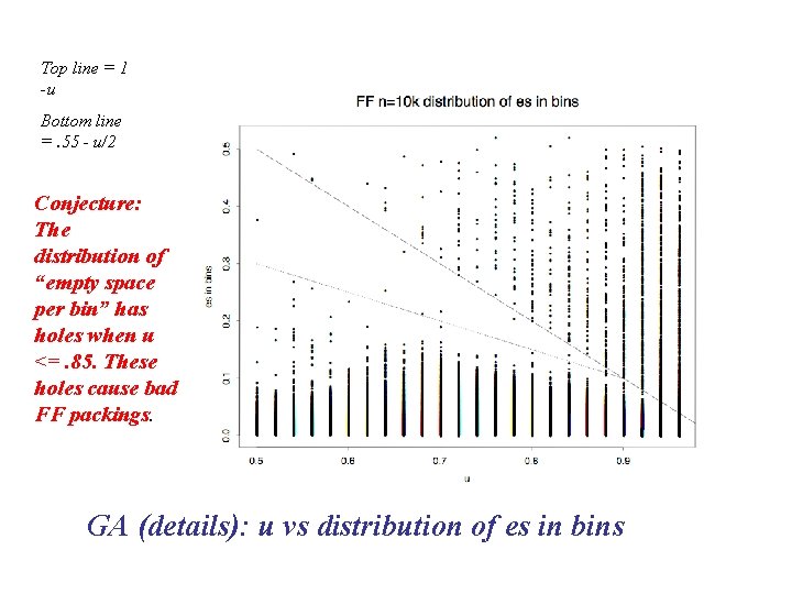
Top line = 1 -u Bottom line =. 55 - u/2 Conjecture: The distribution of “empty space per bin” has holes when u <=. 85. These holes cause bad FF packings. GA (details): u vs distribution of es in bins

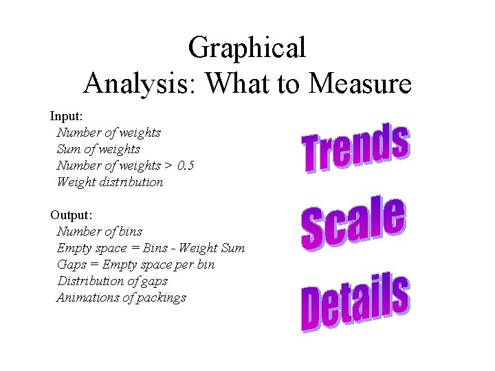
Graphical Analysis: What to Measure Input: Number of weights Sum of weights Number of weights > 0. 5 Weight distribution Output: Number of bins Empty space = Bins - Weight Sum Gaps = Empty space per bin Distribution of gaps Animations of packings

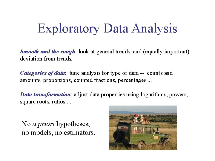
Exploratory Data Analysis Smooth and the rough: look at general trends, and (equally important) deviation from trends. Categories of data: tune analysis for type of data -- counts and amounts, proportions, counted fractions, percentages. . . Data transformation: adjust data properties using logarithms, powers, square roots, ratios. . . No a priori hypotheses, no models, no estimators.

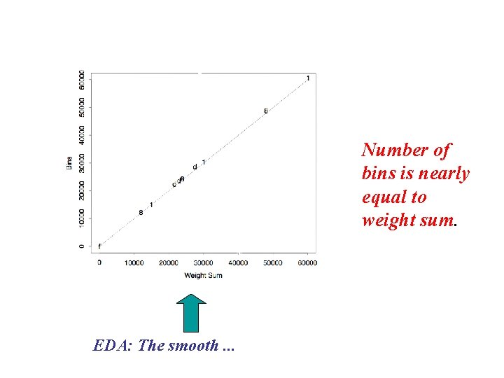
Number of bins is nearly equal to weight sum. EDA: The smooth. . .

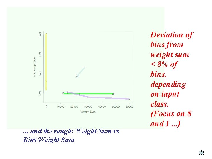
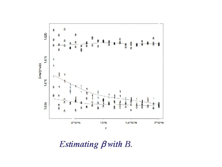
. . . and the rough: Weight Sum vs Bins/Weight Sum Deviation of bins from weight sum < 8% of bins, depending on input class. (Focus on 8 and 1. . . )

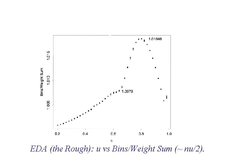
Focus on Uniform Weight Lists Given n weights drawn uniformly from (0, u], for 0 < u <= 1. Consider FF packing quality as f(u), for fixed n.

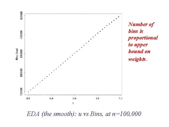
Number of bins is proportional to upper bound on weights. EDA (the smooth): u vs Bins, at n=100, 000

EDA (the Rough): u vs Bins/Weight Sum (~ nu/2).

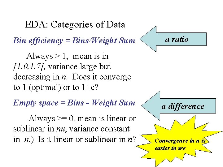
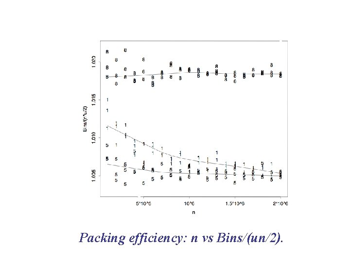
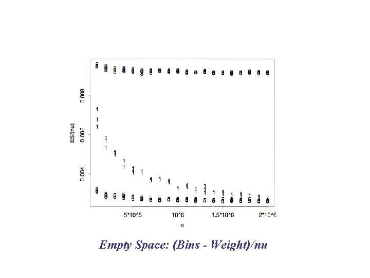
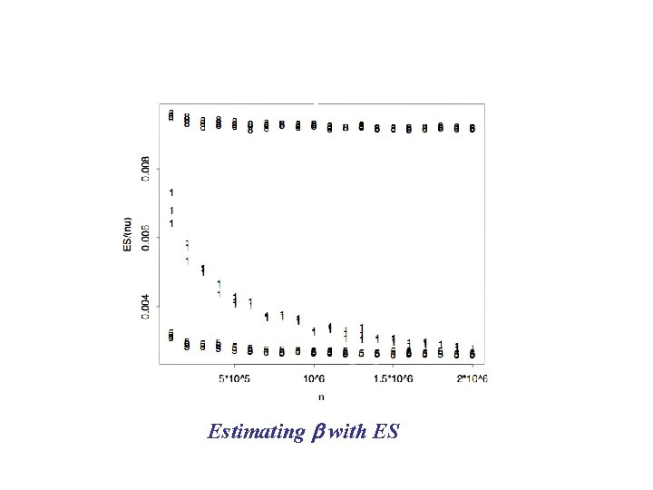
EDA: Categories of Data Bin efficiency = Bins/Weight Sum a ratio Always > 1, mean is in [1. 0, 1. 7], variance large but decreasing in n. Does it converge to 1 (optimal) or to 1+c? Empty space = Bins - Weight Sum Always >= 0, mean is linear or sublinear in nu, variance constant in n. ) Is it linear or sublinear in n? a difference Convergence in n is easier to see

Packing efficiency: n vs Bins/(un/2).

Empty Space: (Bins - Weight)/nu

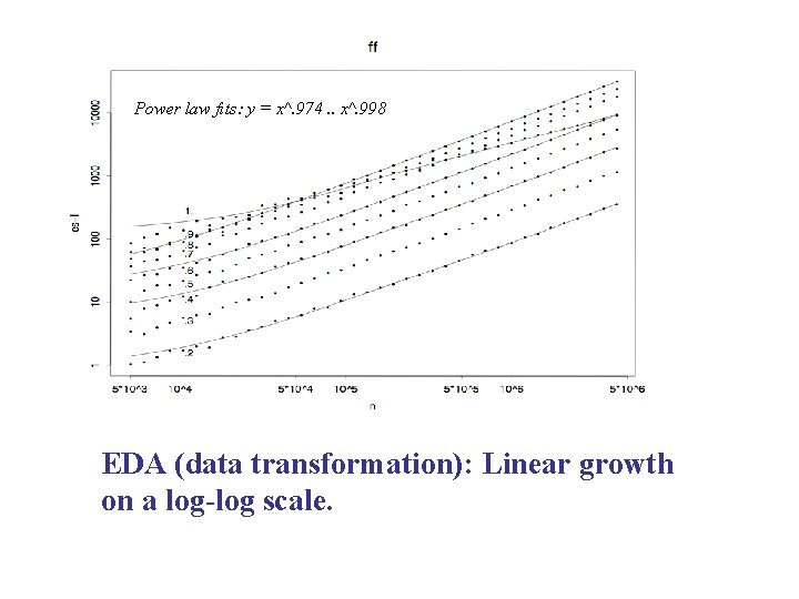
Power law fits: y = x^. 974. . x^. 998 EDA (data transformation): Linear growth on a log-log scale.

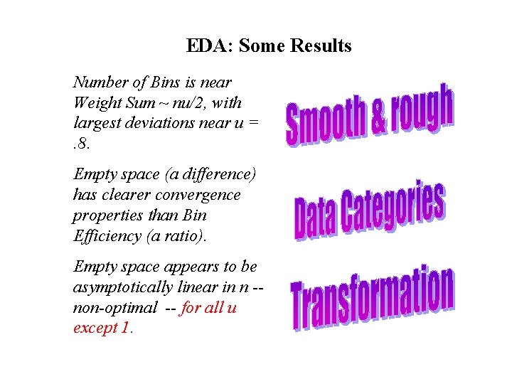
EDA: Some Results Number of Bins is near Weight Sum ~ nu/2, with largest deviations near u =. 8. Empty space (a difference) has clearer convergence properties than Bin Efficiency (a ratio). Empty space appears to be asymptotically linear in n -non-optimal -- for all u except 1.

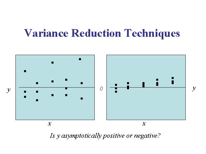
Variance Reduction Techniques y 0 y x x Is y asymptotically positive or negative?

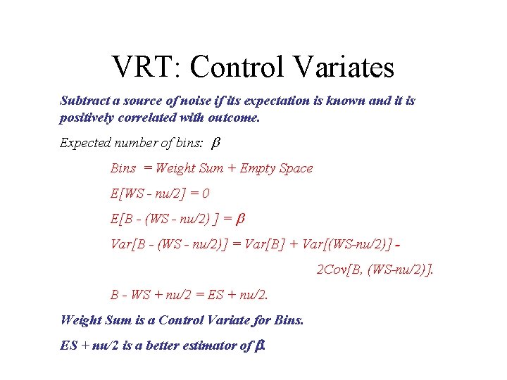
VRT: Control Variates Subtract a source of noise if its expectation is known and it is positively correlated with outcome. Expected number of bins: b Bins = Weight Sum + Empty Space E[WS - nu/2] = 0 E[B - (WS - nu/2) ] = b Var[B - (WS - nu/2)] = Var[B] + Var[(WS-nu/2)] 2 Cov[B, (WS-nu/2)]. B - WS + nu/2 = ES + nu/2. Weight Sum is a Control Variate for Bins. ES + nu/2 is a better estimator of b.

Estimating b with B.

Estimating b with ES

More Variance Reduction Techniques Common Random Variates: Compare heuristics on identical inputs when performance is correlated. Antithetic Variates: Exploit negative correlation in inputs. Stratification: Adjust variations in output according to known variations in input. Conditional Monte Carlo: More data per experiment, using efficient tests.

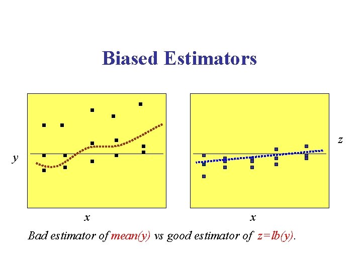
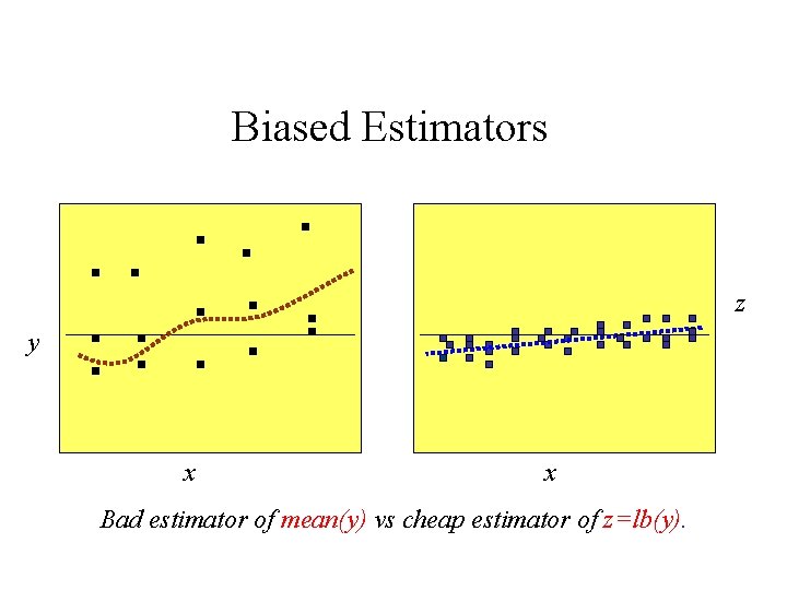
Biased Estimators z y x x Bad estimator of mean(y) vs good estimator of z=lb(y).

Biased Estimators z y x x Bad estimator of mean(y) vs cheap estimator of z=lb(y).

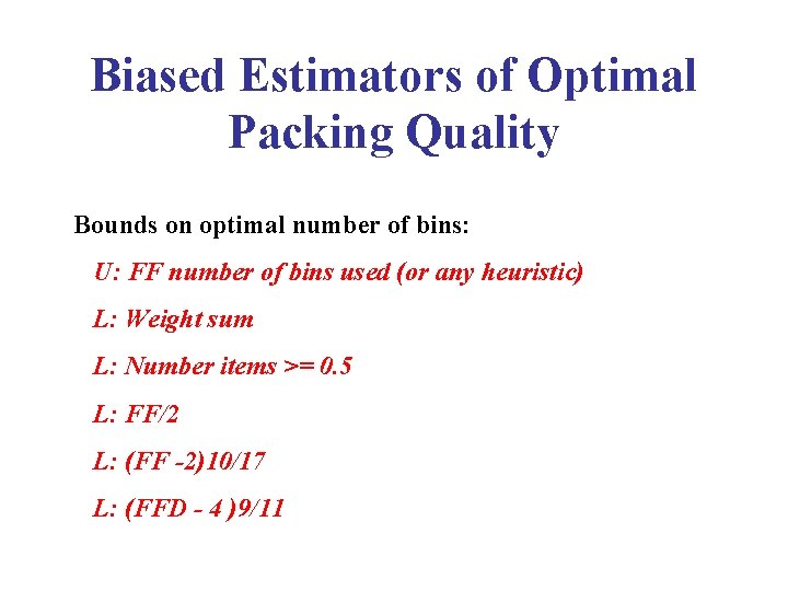
Biased Estimators of Optimal Packing Quality Bounds on optimal number of bins: U: FF number of bins used (or any heuristic) L: Weight sum L: Number items >= 0. 5 L: FF/2 L: (FF -2)10/17 L: (FFD - 4 )9/11

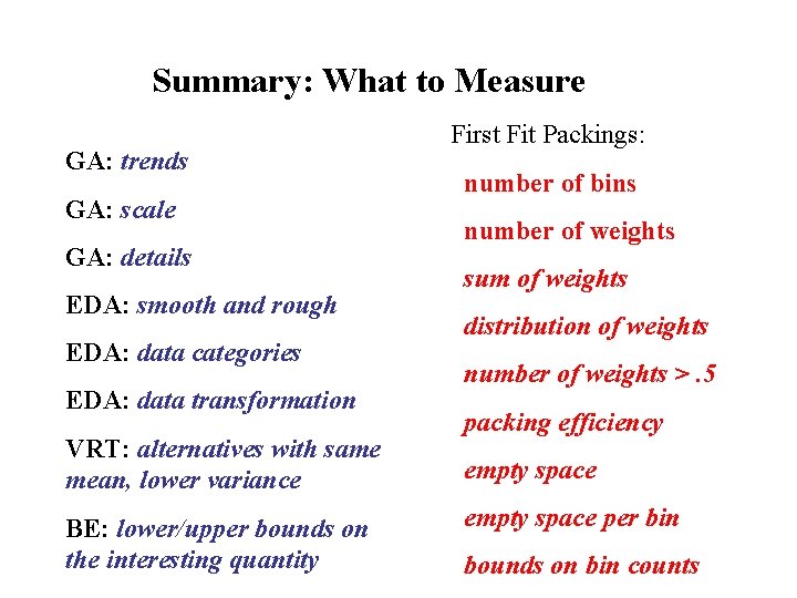
Summary: What to Measure GA: trends GA: scale GA: details EDA: smooth and rough EDA: data categories EDA: data transformation VRT: alternatives with same mean, lower variance BE: lower/upper bounds on the interesting quantity First Fit Packings: number of bins number of weights sum of weights distribution of weights number of weights >. 5 packing efficiency empty space per bin bounds on bin counts

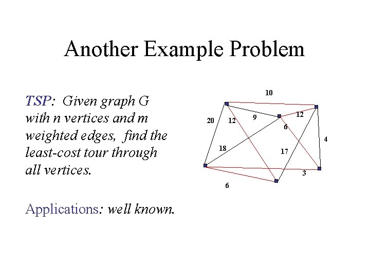
Another Example Problem TSP: Given graph G with n vertices and m weighted edges, find the least-cost tour through all vertices. 10 20 12 6 4 18 17 3 6 Applications: well known. 12 9

TSP: What to Measure VRT’s and BE’s: Mean edge weight is a control variate for Tour Length. Beginning Tour is a control variate for Final Tour, in iterative algorithms with random starts. f(MST + Matching) is a biased estimator of Tour Length (lower bound). Held-Karp Lower Bound is biased estimator of Tour Length. Can you think of others?

TSP: Graphical Analysis Input: Vertices n and Edges m. . . can you think of others? Output: Tour Length. . . can you think of others?

TSP: Exploratory Data Analysis Any ideas?

References Tukey, Exploratory Data Analysis. Cleveland, Visualising Data. Chambers, Cleveland, Kleiner, Tukey, Graphical Methods for Data Analysis. Bratley, Fox, Schrage, A Guide to Simulation. C. C. Mc. Geoch, “Variance Reduction Techniques and Simulation Speedups, ” Computing Surveys, June 1992.

Upcoming Events in Experimental Algorithmics January 2007: ALENEX (Workshop on Algorithm Engineering and Experimentation), New Orleans. Spring 2007: DIMACS/NISS joint workshop on experimental analysis of algorithms, North Carolina. (Center for Discrete Mathematics and Theoretical Computer Science, and National Institute for Statistical Sciences. ) June 2007: WEA (Workshop on Experimental Algorithmics), Rome. (Ongoing): DIMACS Challenge on Shortest Paths Algorithms.

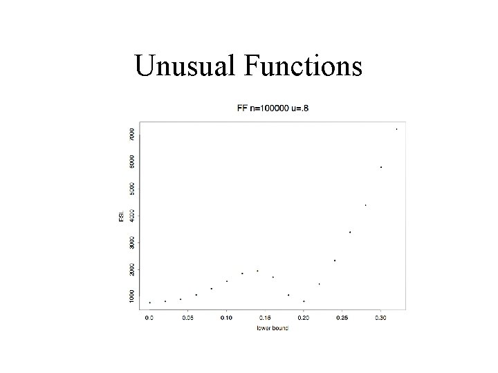
Unusual Functions

EDA: What To Measure The Smooth and the Rough: Bins used is near nu/2, with large deviations in packing quality near u -. 8. Categories of Data: Empty space (a difference) has clearer convergence properties than Bin Efficiency (a ratio). Data Transformation: Empty space appears to be asymptotically linear in n -implying non-optimal convergence -- for all u except 1.

Theory and Practice

Hockey Science: Predict the ingame puck velocities generated by new stick technologies.

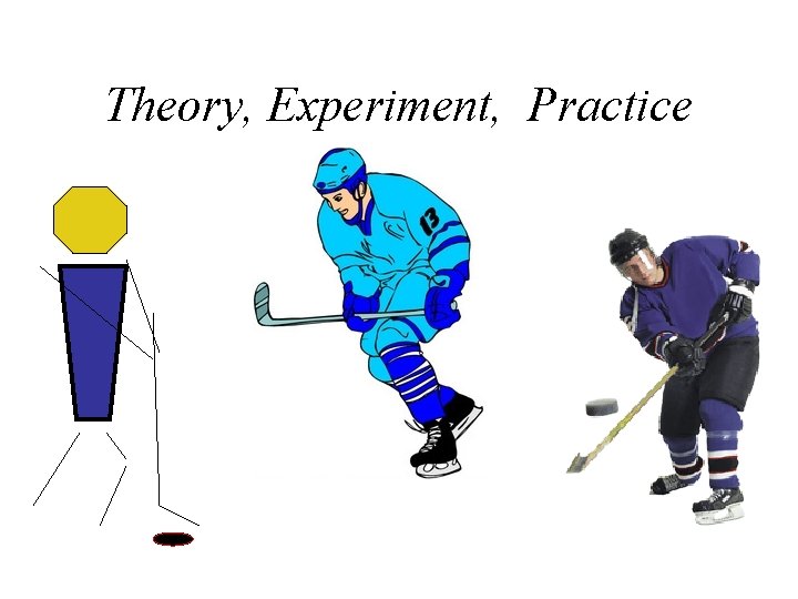
Theory, Experiment, Practice

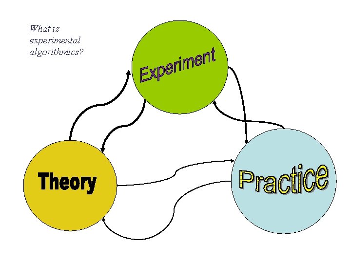
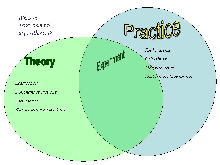
What is experimental algorithmics?

What is experimental algorithmics? Real systems CPU times Measurements Real inputs, benchmarks Abstraction Dominant operations Asymptotics Worst-case, Average Case

First Fit Consider weights in order of arrival; pack each into the first (leftmost) bin that can contain it. u l L = rand_list(n, l, u) S(L)=Sum of weights in L Opt(L) = Optimal number of bins B(L)=Number of bins used in FF ES(L) = Total empty space in bins: B(L) S(L) ESL(L) = Empty space in all but the last bin.

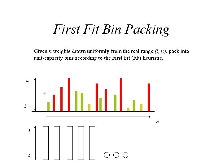
First Fit Bin Packing Given n weights drawn uniformly from the real range (l, u], pack into unit-capacity bins according to the First Fit (FF) heuristic. u + l n 1 0

Type n Bins, Bins/Sum unif file 30, 000 60, 000 120, 000 30, 000 60, 000 15, 270 / 1. 081 30, 446 / 1. 024 60, 809 / 1. 033 9 / 1. 021 13 / 1. 015 file dicto 124, 016 60, 687 61, 406 81, 520 27 / 1. 013 23, 727/ 1. 037 22, 448/1. 047 28, 767/1. 038